NIM simPLEX: A concise scientific Nim library (with CLI and Python binding) providing samplings, uniform grids, and traversal graphs in compositional (simplex) spaces.
Such spaces are considered when an entity can be split into a set of distinct components (a composition), and they play a critical role in many disciplines of science, engineering, and mathematics. For instance, in materials science, chemical composition refers to the way a material (or, more generally, matter) is split into distinct components, such as chemical elements, based on considerations such as fraction of atoms, occupied volume, or contributed mass. And in economics, portfolio composition may refer to how finite capital is split across vehicles, such as cash, equity instruments, real estate, and commodities, based on their monetary value.
Navigation: nimplex (core library) | docs/changelog | utils/plotting | utils/stitching |
Quick Start
If you have a GitHub account, you can get started with nimplex very quickly by just clicking the button below to launch a CodeSpaces environment with everything installed (per instructions in Reproducible Installation section) and ready to go! From there, you can either use the CLI tool (as explained in CLI section) or import the library in Python (as explained in Usage in Python section) and start using it right away. Of course, it also comes with a full Nim compiler and VSCode IDE extensions for Nim, so you can effortlessly modify/extend the source code and re-compile it if you wish.
Installation
There are several easy ways to quickly get nimplex up and running on your system. The choice depends primarily on your preferred way of interacting with the library (CLI, Nim, or Python) and your system configuration.
Pre-Compiled Binaries (quick but not recommended)
If you happen to be on one of the common systems (for which we auto-compile the binaries) and you do not need to modify anything in the source code, you can simply download the latest release from the nimplex GitHub repository and run the executable (nimplex / nimplex.exe) or Python library (nimplex.so / nimplex.pyd) directly just by placing it in your working directory and using it as:
An interactive command line interface (CLI) tool, which will guide you through how to use it if you run it without any arguments like so (on Linux/MacOS):
./nimplexor with a concise configuration defining the task type and parameters (explained later in Usage in Nim):./nimplex -c IFP 3 10
A compiled Python library, which you can import and use in your Python code like so:
import nimplexand immediately use the functions provided by the library, as described in Usage in Python:nimplex.simplex_internal_grid_fractional_py(dim=3, ndiv=10)
Reproducible Installation (recommended)
If the above doesn't work for you, or you want to modify the source code, you can compile the library yourself fairly easily in a couple minutes. The only requirement is to have Nim installed on your system (Installation Instructions) which can be done with a single command on most Unix (Linux/MacOS) systems:
with your distribution's package manager, for instance on Ubuntu/Debian Linux:
apt-get install nim
on MacOS, assuming you have Homebrew installed:
brew install nim
using **conda** cross-platform package manager:
conda install -c conda-forge nim
Then, you can use the bundled Nimble tool (pip-like package manager for Nim) to install two top-level dependencies: arraymancer, which is a powerful N-dimensional array library, and nimpy which helps with the Python bindings. You can do it with a single command:
nimble install -y arraymancer nimpy
Finally, you can clone the repository and compile the library with:
git clone https://github.com/amkrajewski/nimplex
cd nimplex
nim c -r -d:release nimplex.nim --benchmark
which will compile the library and run a few benchmarks to make sure everything runs smoothly. You should then see a compiled binary file nimplex in the current directory which exposes the CLI tool. If you want to use the Python bindings, you can compile the library with slightly different flags (depending on your system configuration) like so for Linux/MacOS:
nim c --d:release --threads:on --app:lib --out:nimplex.so nimplexand you should see a compiled library file nimplex.so in the current directory which can be immediately imported and used in Python.
Capabilities
Note: Full technical discussion of methods and motivations is provided in the manuscript. The sections below are meant to provide a concise overview of the library's capabilities.
The library provides a growing number of methods specific to compositional (simplex) spaces:
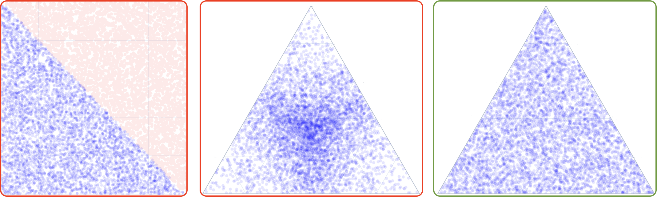
- Monte Carlo sampling is the simplest method conceptually, where points are randomly sampled from a simplex. In low dimensional cases, this can be accomplished by sampling from a uniform distribution in (d-1)-Cartesian space and then rejecting points outside the simplex (left panel below). However, in this approach, the inefficiency growth is factorial with the dimensionality of the simplex space. Instead, some try to sample from a uniform distribution in (d)-Cartesian space and normalize the points to sum to 1, however, this leads to over-sampling in the center of each simplex dimension (middle panel below). One can, however, fairly easily sample from a special case of Dirichlet distribution, as explained in the manuscript, which leads to uniform sampling in the simplex space (right panel below). Nimplex can sample around 10M points per second in 9-dimensional space on a modern CPU.
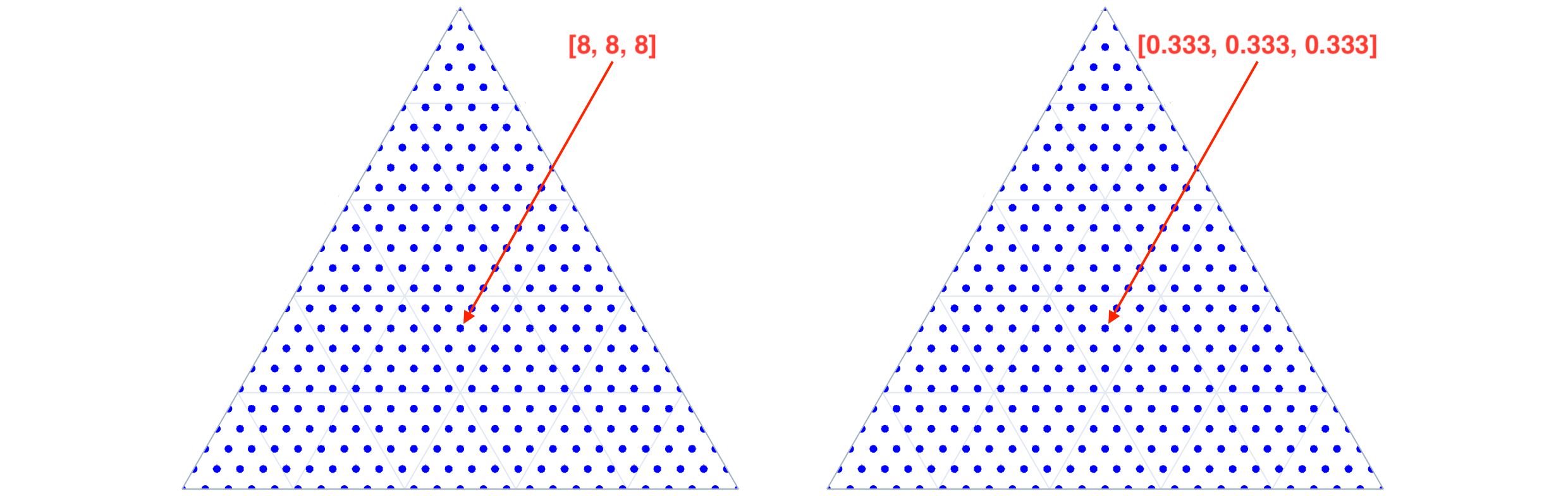
- Simplex / Compositional Grids are a more structured approach to sampling, where all possible compositions quantized to a given resolution, like 1% for 100 divisions per dimension, are generated. This is useful for example when one wants to map a function over the simplex space. In total N_S(d, n_d) = \binom{d-1+n_d}{d-1} = \binom{d-1+n_d}{n_d} are generated, where d is the dimensionality of the simplex space and n_d is the number of divisions per dimension. Nimplex uses a modified version of NEXCOM algorithm to do that procedurally (see manuscript for details) and can generate around 5M points per second in 9-dimensional space on a modern CPU. A choice is given between generating the grid as a list of integer numbers of quantum units (left panel below) or as a list of fractional positions (right panel below).
- Internal Simplex / Compositional Grids are a modification of the above method, where only points inside the simplex, i.e. all components are present, are generated. This is useful in cases where, one cannot discard any component entirely, for instance, because manufacturing setup has minimum feed rate (leakage). Nimplex introduces a new algorithm to generate these points procedurally (see manuscript for details) based on further modification of NEXCOM algorithm. In total N_I(d, n_d) = \binom{n_d-1}{d-1} are generated, critically without any performance penalty compared to the full grid, which can reach orders of magnitude when d approaches n_d. Similar to the full grid, a choice is given between generating the grid as a list of integer numbers of quantum units or as a list of fractional positions.
- Simplex / Compositional Graphs generation is the most critical capability, first introduced in the nimplex manuscript. They are created by using combinatorics and discovered patterns to assign edges between all neighboring nodes during the simplex grid (graph nodes) generation process. Effectively, a traversal graph is generated, spanning all possible compositions (given a resolution) creating an extremely efficient representation of the problem space, which allows deployment of numerous graph algorithms.
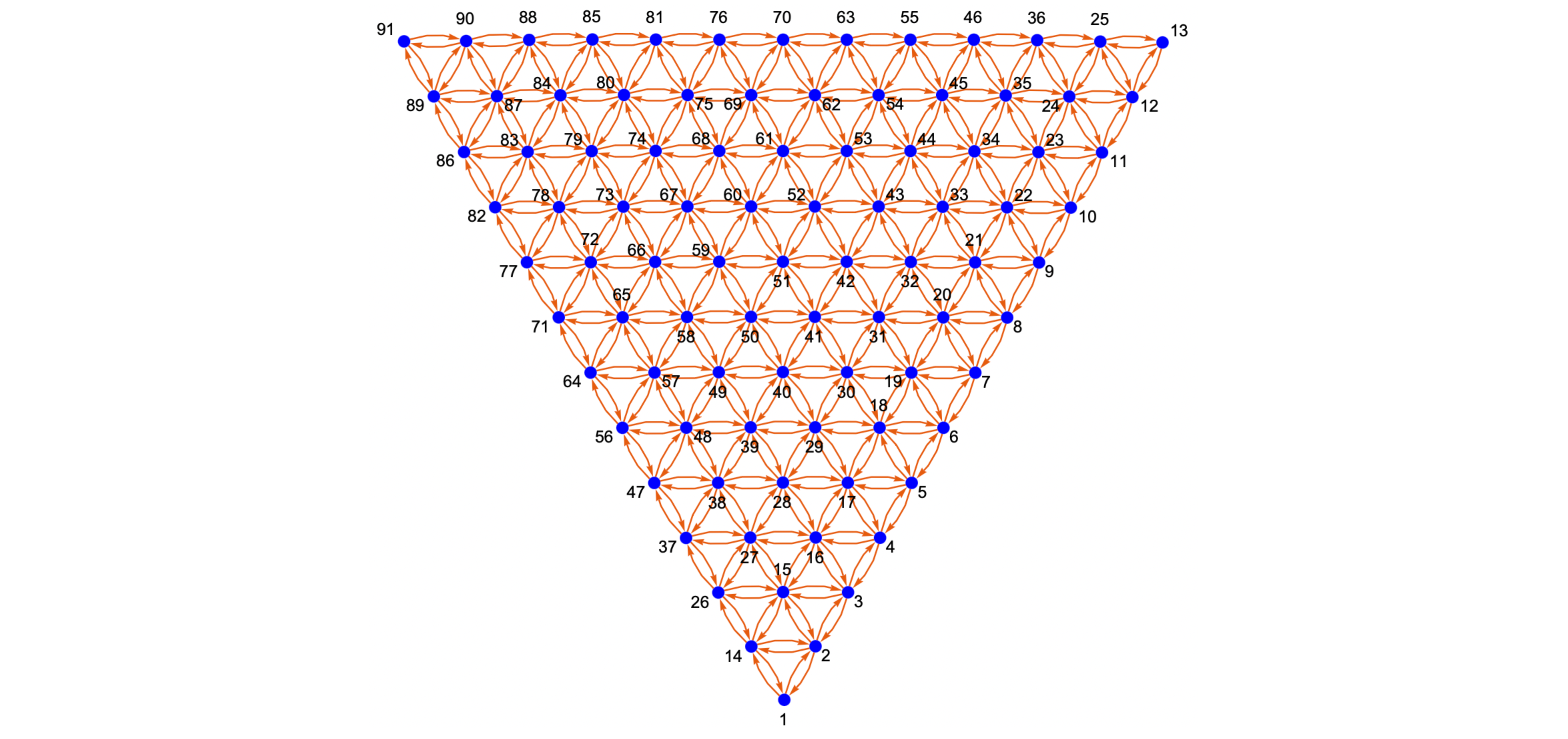
Critically, unlike the O(N^2) distance-based graph generation methods, this approach scales linearly with the resulting number of nodes. Because of that, it is extremely efficient even in high-dimensional spaces, where the number of edges goes into trillions and beyond. Nimplex can both generate and find neighbors for around 2M points per second in 9-dimensional space on a modern CPU.
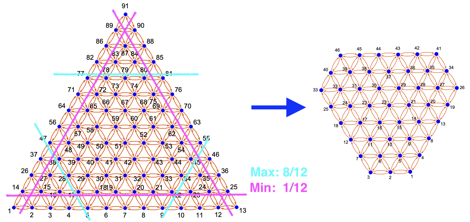
- Limited Simplex / Compositional Graphs where each component (i.e. simplex dimension) can be individually limited by minimum and maximum values, as depicted in the figure below. This allows for efortless creation of graphs representing asymmetric subspaces corresponding to, for instance, “all HEA with at least 5% and at most 55% of each of 8 metallic components but less than 5% of boron and between 4% and 12% of carbon”.
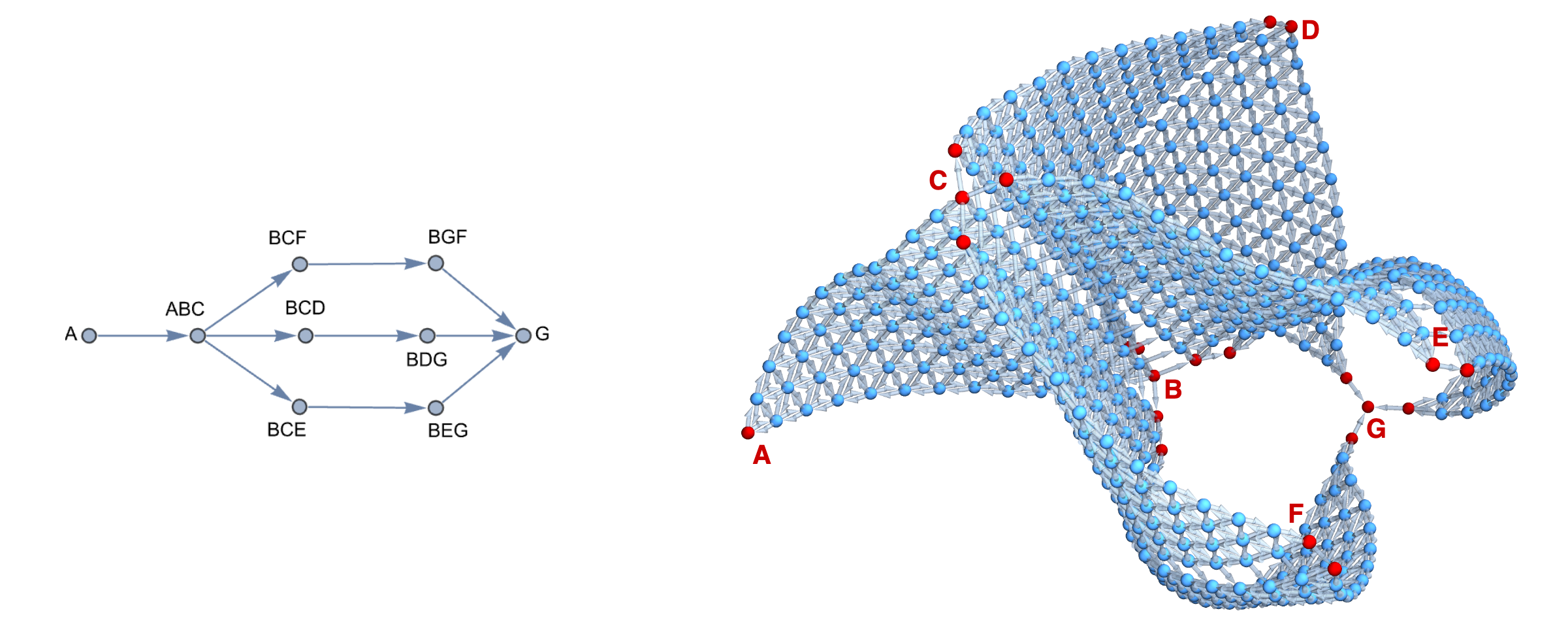
- Graph Complexes, combining multiple individual compositional graphs can also be constructed through the utils/stitching module which computes fixed-orientation subspaces that can be joined together, e.g., A-B-C in A-B-C-D with A-B-C in F-A-C-E-B. As explored in our npj Unconventional Computing article, such combined representations, allowing for even different dimensionalities of joined spaces, can can then be used to efficeintly encode complex problem spaces where some prior assumptions and knowledge are available. In the Example #2 from our article, inspired by problem of joining titanium with stainless steel in 10.1016/j.addma.2022.102649, using 3-component spaces, one can encode 3 separate paths where some components are shared in predetermined fashion. This efficiently encodes the problem space in form of a single simplex graph complex (right panel below) with a single consistent structure, that can be directly used for pathfinding and other graph algorithms just like any other graph.
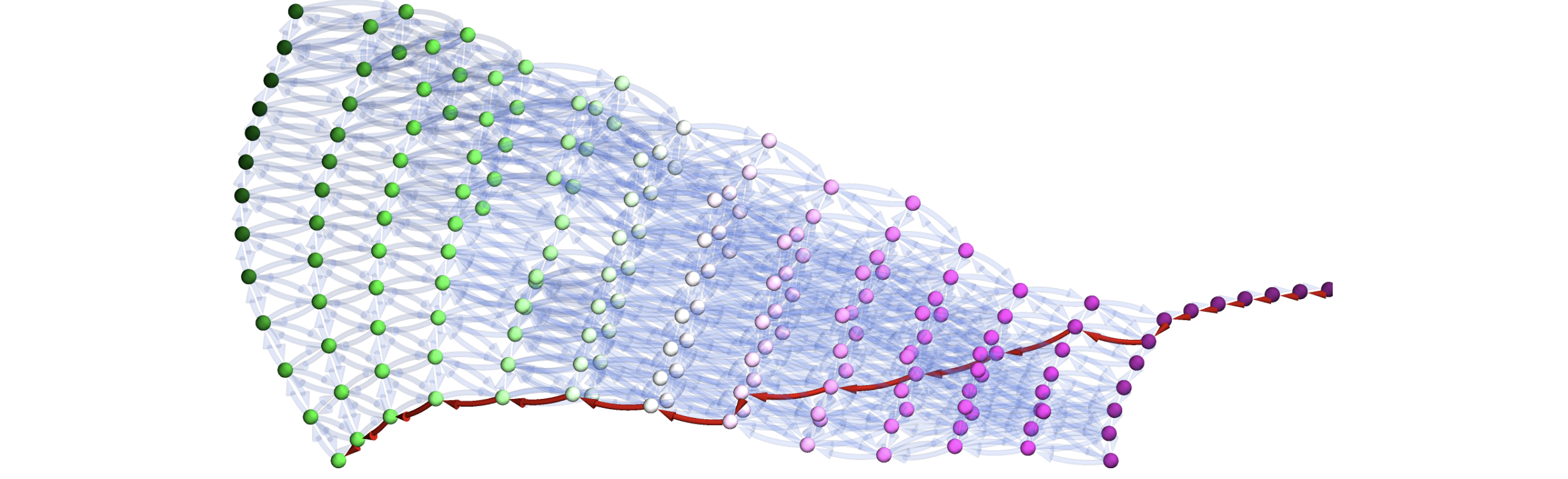
With such graph representation, one can very easily deploy any scientific library for graph exploration, constrained and biased by models operating in the elemental space mapping nimplex provides. A neat and concise demonstration of this is provided in the `02.AdditiveManufacturingPathPlanning.ipynb` under examples directory, where thermodynamic phase stability models constrain a 4-component (tetrahedral) design space existing in 7-component chemical space and property model related to yield strength (RMSAD) is used to bias designed paths towards objectives like property maximization or gradient minimization with extremely concise code simply modifying the weights on unidirectional edges in the graph. For instance, the figure below (approximately) depicts the shortest path through a subset of tetrahedron formed by solid solution phases, later stretched in space proportionally to RMDAS gradient magnitude.
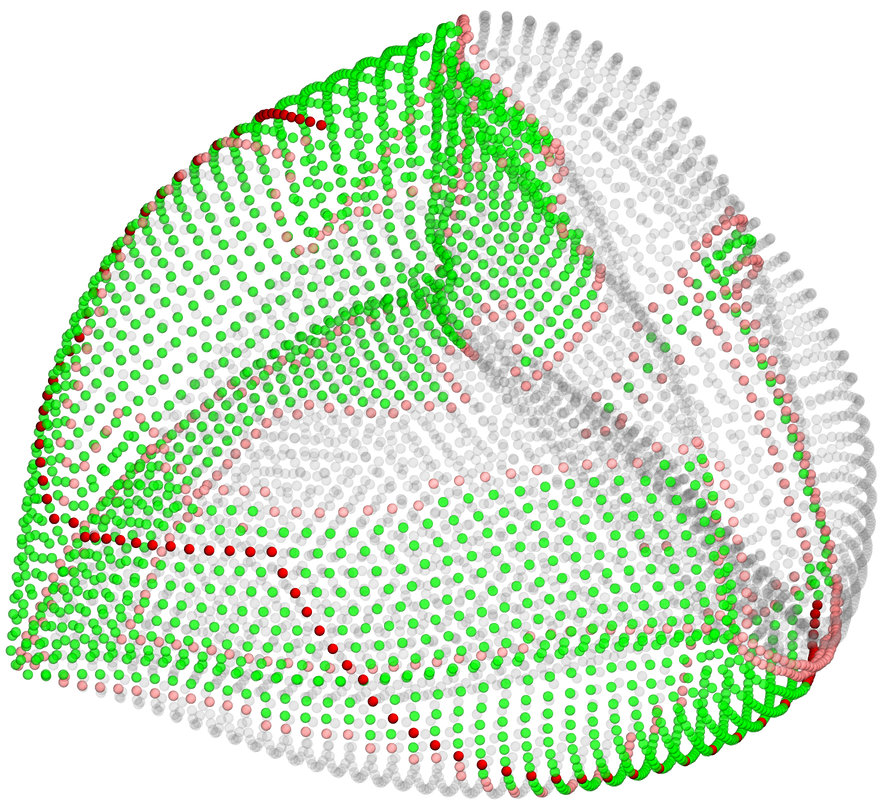
A real-world example of using such context can be found in our paper on AMMap tool, where a graph complex consisting of all possible ternary (3-component) simplex graphs in a 7-component space are joined together, representing a continous space of all possible ternary compositions of 7 elements. In the paper, it is then used to deploy thermodynamic calculations through a search algorithm, with aim of finding the shortest path between two compositions of interest. The resulting graph complex with calculation results overlaid is shown below.
Several other methods are in testing and will likely be added in the future releases. If you have any suggestions, please open an issue on GitHub as we are always soliciting new ideas and use cases based on real-world problems in the scientific computing community.
Usage in Nim
Usage within Nim is fairly straightforward. You can install it using Nimble as explained earlier, or install it directly from GitHub, making sure to use the slightly modified @#nimble branch:
nimble install -y https://github.com/amkrajewski/nimplex@#nimbleor, if you wish to modify the source code, you can simply download the core file nimplex.nim and place it in your own code, as long as you have the dependencies installed, since it is standalone. Then simply follow the API documentation below (please note that it corresponds to the development version, i.e. the current state of the main branch), so some functions may not yet be available in the latest release version.
Usage in Python
To use the library in Python, you can interact with it just like any other Python library. All input/output types are native Python types, so no additional conversion is necessary. Once you have the library installed and imported, simply follow the API documentation below, with an exception that you need to add `_py` to the function names. If you happen to forget adding _py, the Python interpreter will throw an error with a suggestion to do so.
In addition to the bindings, several extra functions cover some higher level use cases, which are not available in Nim because in Nim they can be easily constructed and optimized by the compiler; whereas in Python they would involve type conversions and other overheads when stacked together. These functions are:
proc embeddedpair_simplex_grid_fractional_py(
     components: seq[seq[float]], ndiv: int):
     (seq[seq[float]], seq[seq[float]]) =
Takes the components list of lists of floats, which represents a list of compositions in the elemental space, and ndiv number of divisions per dimension to use when constructing the attainable space. It infers the dimensionality of the attainable space from the length of the components list to construct it, and uses values from components to place each point in the elemental space using attainable2elemental function. The result is a tuple of (1) a seq[seq[float]] of attainable space points and (2) a seq[seq[float]] of elemental space points, both using fractional coordinates (summing to 1).
proc embeddedpair_simplex_internal_grid_fractional_py(
     components: seq[seq[float]], ndiv: int):
     (seq[seq[float]], seq[seq[float]]) =
Same as embeddedpair_simplex_grid_fractional_py but for internal grid. Note that the internal grid does not include the simplex boundary, so the compositions given by components will not be present.
proc embeddedpair_simplex_sampling_mc_py(
     components: seq[seq[float]], samples: int):
     (seq[seq[float]], seq[seq[float]]) =
Same as embeddedpair_simplex_grid_fractional_py but for random sampling (Monte Carlo).
proc embeddedpair_simplex_graph_fractional_py(
     components: seq[seq[float]], ndiv: int):
     (seq[seq[float]], seq[seq[float]], seq[seq[int]]) =
Same as the simplex_graph_fractional but the result tuple now includes a seq[seq[float]] of elemental space points at the second position, while the first position is still a seq[seq[float]] of attainable space points and seq[seq[int]] of neighbor lists for each node is now at the third position
proc embeddedpair_simplex_graph_3C_fractional_py(
     components: seq[seq[float]], ndiv: int):
     (seq[seq[float]], seq[seq[float]], seq[seq[int]]) =
Same as embeddedpair_simplex_graph_fractional_py but for optimized 3-component using simplex_graph_3C_fractional.
CLI
Interactive
Using Nimplex through the CLI relies on the same core library, but provides a simple interface for users who do not want to write any code. It can be used interactively, where the user is guided through the configuration process by just running the executable without any arguments:
./nimplex
Configured
Or it can be run in "configured" mode by using -c or --config flags, followed by a concise configuration defining the task type and parameters. The configuration is a 3-letter string and 2-3 additional parameters, as explained below.
- 3-letter configuration:
- Grid type or uniform random sampling:
- F: Full grid (including the simplex boundary)
- I: Internal grid (only points inside the simplex)
- R: Random/Monte Carlo uniform sampling over simplex.
- G: Graph (list of grid nodes and list of their neighbors)
- L: Limited graph (graph with integer or fractional limits imposed on the compositions)
- Fractional or Integer positions:
- F: Fractional grid/graph (points are normalized to fractions of 1)
- I: Integer grid/graph (points are integers)
- Print full result, its shape, or persist in a file:
- P: Print (presents full result as a table)
- S: Shape (only the shape / size information)
- N: Persist to NumPy array file ("nimplex_<configFlags>.npy" or optionally a custom path as an additonal argument)
- Grid type or uniform random sampling:
- Simplex Dimensions / N of Components: An integer number of components in the simplex space.
- N Divisions per Dimension / N of Samples: An integer number of either:
- Divisions per each simplex dimension for grid or graph tasks (F/I/G/L__)
- Number of samples for random sampling tasks (R__)
- (for limited graphs only) Limits: A string list of pairs of either integers or floats, depending on the grid type specified by the second letter of the configuration string. Each pair represents the minimum and maximum values for each simplex dimension. The number of pairs must match the number of simplex dimensions. You can use [, {, or @[ for the list. E.g., [[0, 1],[0,0.555],[0.222,0.888]] for fractional grid limits or {{0,12},{2,10},{3,9}} for integer grid limits. Setting the limits to less than 0 or greater than 1/nDiv will pass with a warning, but will not throw an error. The integer limits are exactly inclusive, while the fractional limits inclusive of the closeset grid point, i.e. max limit of 0.660 will let 1/3=0.667 pass for low resolution grids, but not high resolution ones.
- (optional) NumPy Array Output Filename: A custom path to the output NumPy array file (only for __N tasks).
For instance, to generate a 3-dimensional internal fractional grid with 10 divisions per dimension and persist it to a NumPy array file, you can run:
./nimplex -c IFN 3 10and the output will be saved to nimplex_IF_3_10.npy in the current directory. If you want to save it to a different path, you can provide it as an additional argument:
./nimplex -c IFN 3 10 path/to/outfile.npyOr if you want to print the full result to the console, allowing you to pipe it to virtually any other language or tool as plain text, you can run:
./nimplex -c IFP 3 10
Auxiliary Flags
You can also utilize the following auxiliary flags:
- --help or -h --> Show help.
- --benchmark or -b --> Run a set of tasks to benchmark performnace (simplex_grid(9, 12), simplex_internal_grid(9, 12), simplex_sampling_mc(9, 1_000_000), simplex_graph(9, 12)) and compare performance across implementations (simplex_graph(3, 1000) vs simplex_graph_3C(1000)).
API
The following sections cover the core API of the library. Further documentation for auxiliary functions, defined in utils submodule, can be found by following links under Imports below or by searching the API Index in the top left corner of this page.
Lets
args = commandLineParams()
- Command line arguments parsed when the module is run as a script, rather than as a library, allowing efortless CLI usage without any Python or Nim knowledge. When empty, interactive mode is triggered and user is navigated through the configuration process. Otherwise, the first argument is expected to be -c or --config followed by the configuration flags and parameters as described in the help message below. See echoHelp() for more details. Source Edit
Procs
proc attainable2elemental(simplexPoints: Tensor[SomeNumber];
                          components: seq[seq[SomeNumber]]): Tensor[float]
-
Projects each point from the attainable space to the elemental space using matrix multiplication. Accepts a simplexPoints Arraymancer Tensor[float] or Tensor[int] of shape corresponding to a simplex grid (e.g., from simplex_grid_fractional) or random samples (e.g., from simplex_sampling_mc) and a components list of lists of floats or ints, which represents a list of compositions in the elemental space serving as base components of the attainable space given in simplexPoints. The components can be a row-consistnet mixed list list of integer and fractional compositions, and will be normalized per-row to allow for both types of inputs. Please note that it will not automatically normalize the simplexPoints rows, so if you give it integer compositions, you will get float values summing to ndiv rather than 1.
Example:
import arraymancer/Tensor
const components = @[
    @[0.94, 0.05, 0.01], # Fe95 C5 Mo1
    @[3.0, 1.0, 0.0],    # Fe3C
    @[0.2, 0.0, 0.8]     # Fe20 Mo80
]
let grid = simplex_grid_fractional(3, 4)
let elementalGrid = grid.attainable2elemental(components)
echo elementalGrid
# Tensor[system.float] of shape "[15, 3]" on backend "Cpu"
# |0.2            0       0.8|
# |0.3375    0.0625       0.6|
# |0.475      0.125       0.4|
# |0.6125    0.1875       0.2|
# |0.75        0.25         0|
# |0.385     0.0125    0.6025|
# |0.5225     0.075    0.4025|
# |0.66      0.1375    0.2025|
# |0.7975       0.2    0.0025|
# |0.57       0.025     0.405|
# |0.7075    0.0875     0.205|
# |0.845       0.15     0.005|
# |0.755     0.0375    0.2075|
# |0.8925       0.1    0.0075|
# |0.94        0.05      0.01|
Source Edit func configValidation(config: string) {....raises: [], tags: [], forbids: [].}
- Validates the 3-letter configuration string provided by the user. Source Edit
proc elemental_space_scaling_table(components: seq[seq[float]]): Table[seq[int],
    float] {....raises: [], tags: [], forbids: [].}
-
Generates a scaling table for converting unit distances in the attainable simplex space to elemental distances in the elemental space (e.g., in atomic percent changes in
some chemical spaces), which are mathematically the same as half of Manhattan distances (i.e. [0.25, 0.75, 0.0] to [0.0, 1.0, 0.0] is 0.25 distance because chaning the
composition requires changing 25% A to B). The resulting table maps from all N*(N-1)/2 possible senseless direction / lines, expressed as two-hot `seq[int]` of length N
(e.g., for N=3, `[1,1,0]`, `[1,0,1]`, and `[0,1,1]`), to the corresponding distance scaling factor in the elemental space.
Example:
const components = @[
    @[0.94, 0.05, 0.01], # Fe95 C5 Mo1
    @[3.0, 1.0, 0.0],    # Fe3C
    @[0.2, 0.0, 0.8]     # Fe20 Mo80
]
echo elemental_space_scaling_table(components)
# {
#  @[1, 1, 0]: 0.2,
#  @[1, 0, 1]: 0.79,
#  @[0, 1, 1]: 0.8
# }
Source Edit func nDivValidation(config: string; nDiv: int; dim: int) {....raises: [], tags: [], forbids: [].}
- Validates the number of divisions per each simplex dimension provided by the user for all tasks except Random sampling. Source Edit
proc outFunction(config: string; npyName: string; outputData: Tensor)
- Handles the output of a simplex grid or random sampling in outputData Tensor when run from the CLI, based on the 3rd letter of the configuration string config, and the destiantion filename npyName, which should include the extension. Source Edit
proc outFunction_graph(config: string; dim: int; ndiv: int; npyName: string;
                       outputData: (Tensor, seq))
- Handles the output of graph tasks when run from the CLI, based on the 3rd letter of the configuration string config, the number of dimensions dim, the number of divisions per dimension ndiv, which together are used to determine the graph edges Tensor shape (using math) faster than querying the input edges sequence. The destiantion filename npyName, which should include the extension, also needs to be provided. Source Edit
proc parseLimitFloats(s: string): seq[seq[float]] {.
    ...raises: [RegexError, ValueError], tags: [], forbids: [].}
- Parses a CLI input string containing single nested lists of floats into a sequence of sequences of floats. The input string can contain lists in the form of [], {}, or @[] and can include negative numbers. Source Edit
proc parseLimitInts(s: string): seq[seq[int]] {.
    ...raises: [RegexError, ValueError], tags: [], forbids: [].}
- Parses a CLI input string containing single nested lists of integers into a sequence of sequences of integers. The input string can contain lists in the form of [], {}, or @[] and can include negative numbers. Source Edit
func pure_component_indexes(dim: int; ndiv: int): seq[int] {....raises: [],
    tags: [], forbids: [].}
-
This helper function returns a seq[int] of indexes of pure components in a simplex grid of dim dimensions and ndiv divisions per dimension (e.g., from simplex_grid).
Example:
echo "A B C pure components at indices: ", pure_component_indexes(3, 12)
# A B C pure components at indices: @[90, 12, 0]
Source Edit func pure_component_indexes_internal(dim: int; ndiv: int): seq[int] {. ...raises: [], tags: [], forbids: [].}
-
This helper function returns a seq[int] of indexes of pure components in an internal simplex grid of dim dimensions and ndiv divisions per dimension (e.g., from simplex_internal_grid). In this context, by pure components we mean corners of the simplex, corresponding to the points where one component is at its maximum and all others are at exactly one quanta (e.g., 1/ndiv).
Example:
echo "A+B1C1 B+A1C1 C+A1B1 pure components at indices: ", pure_component_indexes_internal(3, 12)
# A+B1C1 B+A1C1 C+A1B1 pure components at indices: @[54, 10, 0]
Source Edit proc simplex_graph(dim: int; ndiv: int): (Tensor[int], seq[seq[int]]) {. ...raises: [], tags: [], forbids: [].}
-
Generates a simplex graph in a dim-component space based on (1) grid of nodes following ndiv divisions per dimension (i.e., quantized to 1/ndiv), similar to simplex_grid, and (2) a list of neighbor lists corresponding to edges. The result is a tuple of (1) a deterministically allocated Arraymancer Tensor[int] of shape (N_S(dim, ndiv), dim) containing all possible compositions in the simplex space just like in simplex_grid, and (2) a seq[seq[int]] containing a list of neighbors for each node. The current implementation utilizes GC-allocated seq for neighbors to reduce memory footprint in cases where ndiv is close to dim and not all nodes have the complete set of dim(dim-1) neighbors. This is a tradeoff between memory and performance, which can be adjusted by switching to a (N_S(dim, ndiv), dim(dim-1)) Tensor[int] with -1 padding for missing neighbors, just like done in outFunction_graph for NumPy output generation.
Example:
import arraymancer/Tensor
let (nodes, neighbors) = simplex_graph(3, 4)
let nodeSequence = nodes.toSeq2D()
for i in 0..<nodeSequence.len:
    echo i, ":  ", nodeSequence[i], " -> ", neighbors[i]
# 0:  @[0, 0, 4] -> @[1, 5]
# 1:  @[0, 1, 3] -> @[0, 2, 5, 6]
# 2:  @[0, 2, 2] -> @[1, 3, 6, 7]
# 3:  @[0, 3, 1] -> @[2, 4, 7, 8]
# 4:  @[0, 4, 0] -> @[3, 8]
# 5:  @[1, 0, 3] -> @[1, 0, 6, 9]
# 6:  @[1, 1, 2] -> @[2, 1, 5, 7, 9, 10]
# 7:  @[1, 2, 1] -> @[3, 2, 6, 8, 10, 11]
# 8:  @[1, 3, 0] -> @[4, 3, 7, 11]
# 9:  @[2, 0, 2] -> @[6, 5, 10, 12]
# 10:  @[2, 1, 1] -> @[7, 6, 9, 11, 12, 13]
# 11:  @[2, 2, 0] -> @[8, 7, 10, 13]
# 12:  @[3, 0, 1] -> @[10, 9, 13, 14]
# 13:  @[3, 1, 0] -> @[11, 10, 12, 14]
# 14:  @[4, 0, 0] -> @[13, 12]
Source Edit proc simplex_graph_3C(ndiv: int): (Tensor[int], seq[seq[int]]) {....raises: [], tags: [], forbids: [].}
- A special case of simplex_graph for 3-component spaces, which is optimized for performance by avoiding the use of binom function and filling the neighbor list sequentially only once per node (in both directions). Source Edit
proc simplex_graph_3C_fractional(ndiv: int): (Tensor[float], seq[seq[int]]) {.
    ...raises: [ValueError], tags: [], forbids: [].}
- A special case of simplex_graph_fractional for 3-component spaces utilizing optimized simplex_graph_3C. Source Edit
proc simplex_graph_fractional(dim: int; ndiv: int): (Tensor[float],
    seq[seq[int]]) {....raises: [ValueError], tags: [], forbids: [].}
- Conceptually similar to simplex_graph but the first part of the result tuple (graph nodes) is an Arraymancer Tensor[float] of shape (N_S(dim, ndiv), dim) containing all possible compositions in the simplex space expressed as fractions summing to 1 (same as simplex_grid_fractional). Source Edit
proc simplex_graph_limited(dim: int; ndiv: int; limit: seq[seq[int]]): (
    Tensor[int], seq[seq[int]]) {....raises: [ValueError], tags: [], forbids: [].}
-
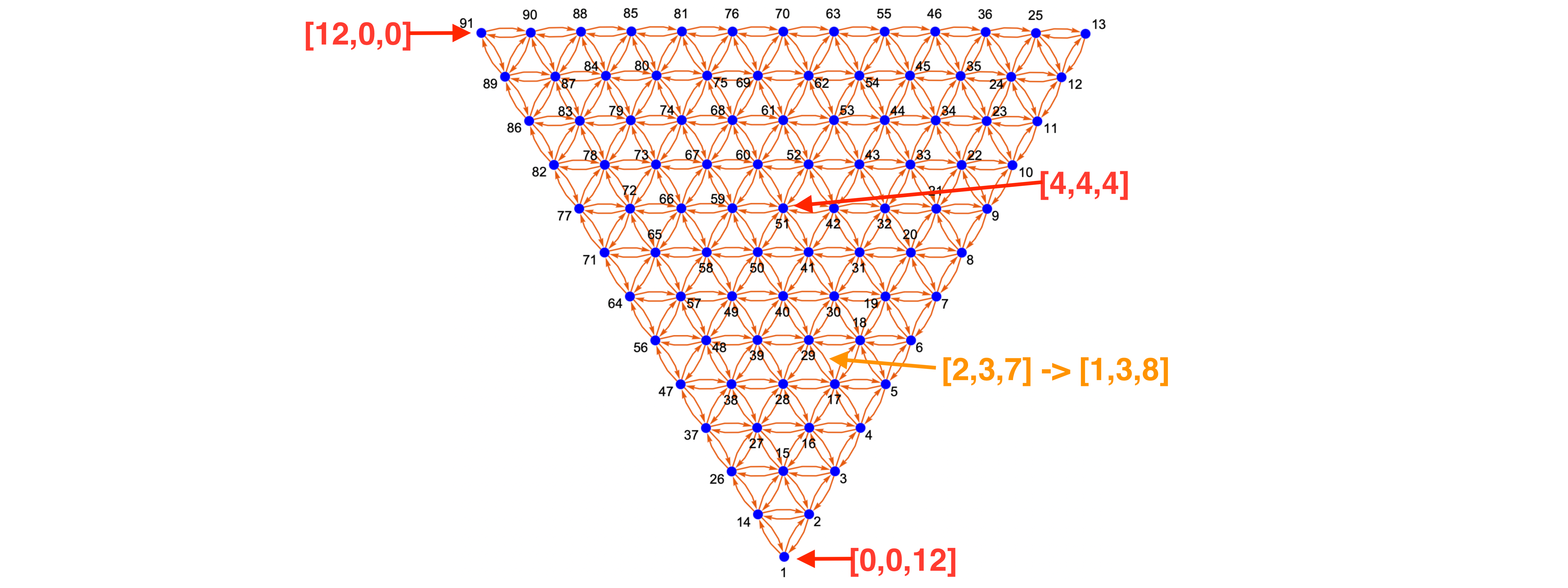
Generates a "limited" simplex graph in up to dim-component space represented by (1) grid of nodes quantized to 1/ndiv, similar to simplex_grid, and (2) a list of neighbor lists corresponding to edges, but only for nodes within the specified limit sequence of integer pairs denoting maximum and minimum values for each component in terms of fractions of ndiv (e.g. [[0, 24], [0, 12], [3, 6]] with ndiv=24 would mean that the first component can take values from 0 to 100%, the second from 0 to 50%, and the third from 12.5 to 25%, inclusive). The figure above depicts an example of a 3-component simplex graph with ndiv=12 and limits of [[1, 8], [1, 8], [1, 8]]. This implementation iterates over all nodes but only computes neighbors for those within the limits, which then gets prunned to avoid connecting to nodes outside the limits (difficult to avoide for more than 3 components). The is rearranged and node indexes are remapped to be a dense uniformly spread grid in a subspace of the simplex, akin to the full simplex_graph but with a smaller number of nodes and more elaborate shapes, such as in the figure below with ndiv=24 and limits of [[0, 24], [0, 24], [0, 12], [0, 3]], resulting in a tetrahedron cut around its base and one corner.
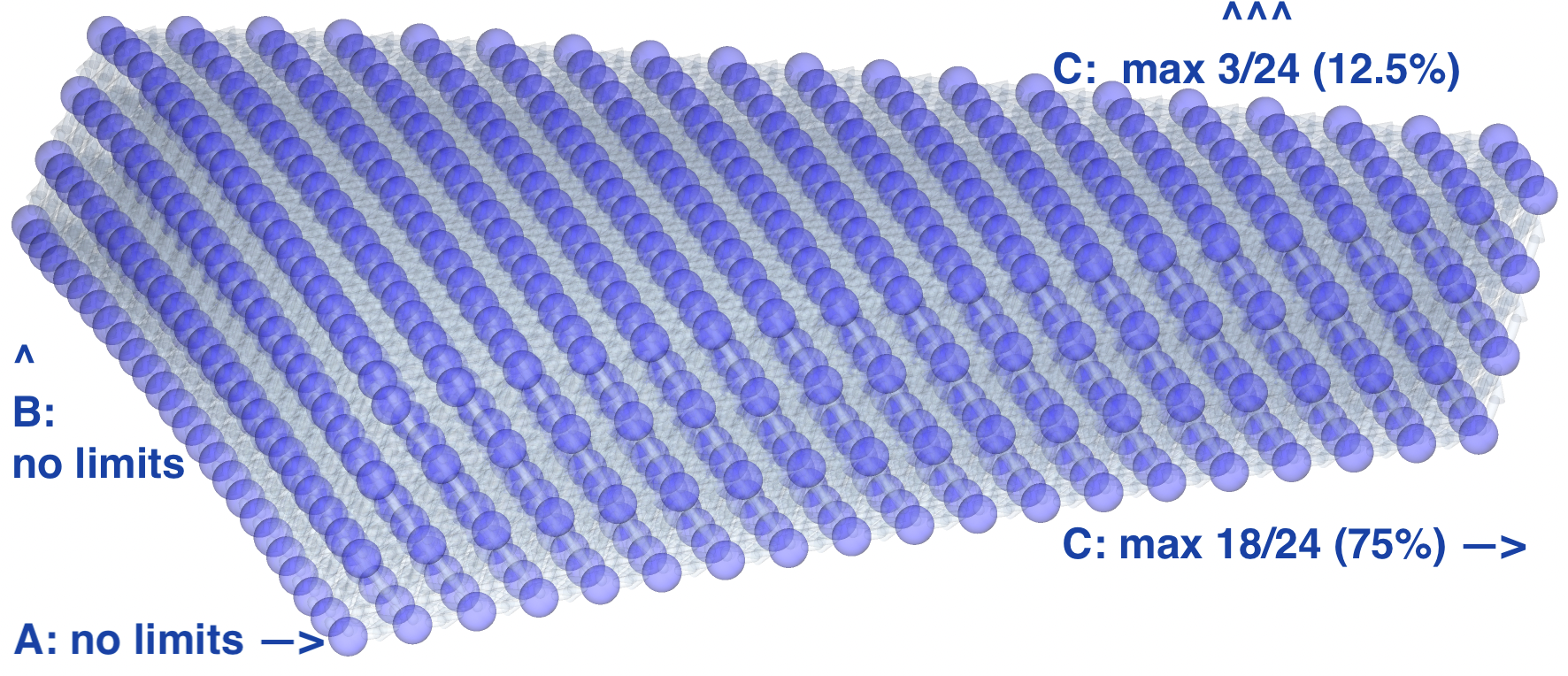
The result is a tuple of (1) a runtime allocated Arraymancer Tensor[int] of shape (N<=N_S(dim, ndiv), dim) containing compositions and (2) a seq[seq[int]] containing a list of neighbors for each node.
Source Edit proc simplex_graph_limited_fractional(dim: int; ndiv: int; limit: seq[seq[float]]): (Tensor[float], seq[seq[int]]) {....raises: [ValueError], tags: [], forbids: [].}
- Similar to simplex_graph_limited but both the limit and the result are fractional (float fraction of 1) rather than integer (quantized to 1/ndiv). Importantly, to avoid issues with floating point precission (e.g. max limit of 0.666 excluding point at 2/3), the limit passed to this function is quantized to the nearest 1/ndiv value, so it will not be applied exactly but rather depend on the ndiv set. For instance max limit of 0.66 will include the exact 2/3 if ndiv is a multiple of 3 or 24, but not if ndiv is 99 as 65/99 is closer than 66/99. At the same time, with ndiv of 10 or 13, points slightly above the limit, namely 7/10 and 9/13 will be included in the graph. Source Edit
proc simplex_grid(dim: int; ndiv: int): Tensor[int] {....raises: [], tags: [],
    forbids: [].}
-

Generates a full (including the simplex boundary) simplex grid in a dim-component space with ndiv divisions per dimension (i.e., quantized to 1/ndiv). The result is a deterministically allocated Arraymancer Tensor[int] of shape (N_S(dim, ndiv), dim) containing all possible compositions in the simplex space expressed as integer numbers of quantum units. The grid is generated procedurally using a modified version of NEXCOM algorithm (see manuscript for details).
Source Edit proc simplex_grid_fractional(dim: int; ndiv: int): Tensor[float] {. ...raises: [ValueError], tags: [], forbids: [].}
-

Conceptually similar to simplex_grid but results in Arraymancer Tensor[float] of shape (N_S(dim, ndiv), dim) containing all possible compositions in the simplex space expressed as fractions summing to 1. The grid is generated procedurally using a modified version of NEXCOM algorithm (see manuscript for details) and then normalized to 1 in a quick single-pass post-processing step.
Source Edit proc simplex_internal_grid(dim: int; ndiv: int): Tensor[int] {....raises: [], tags: [], forbids: [].}
- Same as simplex_grid but generates only points inside the simplex, i.e., all components are present. Source Edit
proc simplex_internal_grid_fractional(dim: int; ndiv: int): Tensor[float] {.
    ...raises: [ValueError], tags: [], forbids: [].}
- Conceptually similar to simplex_internal_grid but results in Arraymancer Tensor[float] of shape (N_I(dim, ndiv), dim) containing all possible compositions in the simplex space expressed as fractions summing to 1 (same as simplex_grid_fractional). Source Edit
proc simplex_sampling_mc(dim: int; samples: int): Tensor[float] {.
    ...raises: [ValueError], tags: [], forbids: [].}
- Randomly samples samples number of points from a simplex in a dim-component space. The result is a deterministically allocated Arraymancer Tensor[float] of shape (samples, dim) containing all sampled points expressed as fractions summing to 1. As eluded to in Capabilities, this is not as straightforward as in Euclidean spaces. The sampling is done by generating samples number of points from a special case of Dirichlet distribution (alpha=1) by sampling from a uniform distribution in (dim)-Cartesian space, then taking the negative logarithm of each coordinate, and finally normalizing each point to sum to 1. This approach is described in the manuscript and contrasted with another (lower performance) approach involving sorting. Source Edit
proc taskRouter(config: string; dim: int; ndiv: int; npyName: string;
                limit: string): void {....raises: [ValueError, IOError, OSError,
    RegexError], tags: [WriteIOEffect], forbids: [].}
- Routes the task to the appropriate calculation and output function based on the first 2 letters of the configuration string. Source Edit
Templates
template benchmark(benchmarkName: string; code: untyped)
- A simple benchmarking template which takes a name and a code block to run. It prints the benchmark name and the duration of the code block execution in natural time units quantized to microseconds (e.g., 119 milliseconds and 296 microseconds). All tasks together should take 500-1000 milliseconds on a modern CPU. Source Edit