| Main Page | Lecture 1 (native render) | Lecture 2 (native render) |
# Introduction
In this guest lecture, we will cover:
- Manipulating and analyzing materials - using pymatgen
- Setting up a small NoSQL database on the cloud to synchronize decentralized processing - using MongoDB Atlas Free Tier
- Interacting with the database - using pymongo library
- Installing machine learning (ML) tools to predict stability of materials - using pySIPFENN
# Before you Start Running This Notebook
Before you begin, you will need to set up a few essential development tools.
While not required, it is recommended first to set up a virtual environment using venv or Conda. This ensures that one of the required versions of Python (3.9+) is used and there are no dependency conflicts. It often comes preinstalled, like in GitHub Codespaces and some Linux distributions. You can quickly check that by running.
conda --version
And if it is not installed, you can follow the (miniconda instructions ) for a quick clean setup.
Once you have Conda installed on your system, you can create a new environment with:
conda create -n 580demo python=3.10 jupyter numpy scipy
conda init
Restart your terminal, and activate the environment with:
conda activate 580demo
At this point, you should be able to run jupyter notebook and open this notebook in your browser with it or select the kernel 580demo in VS Code (top-right corner) or other IDEs.
# Now you are ready to start!
First, we will import some libraries that ship with Python so that we don't need to worry about getting them, and are used in this notebook:
from pprint import pprint            # pretty printing
from collections import defaultdict  # convenience in the example
import os                            # file handling
from datetime import datetime        # time handling
from zoneinfo import ZoneInfo        # time handling
Now, we need to use pip package manager to install the rest of the libraries we will use. If you are using Conda, you could also use conda install instead, but it is more elaborate for non-Anaconda-default packages.
We start with pymatgen, used in the next part of this notebook. To install it, simply remove the # in the following line and run it, or open a terminal and run pip install pymatgen without neither # nor !.
#!pip install pymatgen
And then install pymongo used in the 2nd part:
#!pip install pymongo
Now, you should be ready to go!
# Manipulating and analyzing materials
To start working with atomic structures, often referred to as atomic configurations or simply materials, we must be able to represent and manipulate them. One of the most powerful and mature tools to do so is pymatgen, which we just installed. The critical component of pymatgen is its library of representations of fundamental materials objects, such as Structure and Molecule, contained in the pymatgen.core module. Let's import it and create a simple cubic structure of Al just as we did in the DFTTK tutorial last week:
# Basics
from pymatgen.core import Structure

s = Structure(lattice=[[4.0384, 0, 0], [0, 4.0384, 0], [0, 0, 4.0384]],
              species=['Al', 'Al', 'Al', 'Al'],
              coords=[[0.0, 0.0, 0.0], [0, 0.5, 0.5], [0.5, 0.0, 0.5], [0.5, 0.5, 0.0]])
Now, s holds our initialized structure, and we can apply print on it to see what it looks like:
print(s)
Full Formula (Al4)
Reduced Formula: Al
abc   :   4.038400   4.038400   4.038400
angles:  90.000000  90.000000  90.000000
pbc   :       True       True       True
Sites (4)
  #  SP      a    b    c
---  ----  ---  ---  ---
  0  Al    0    0    0
  1  Al    0    0.5  0.5
  2  Al    0.5  0    0.5
  3  Al    0.5  0.5  0
Initialized is a critical word here because the Structure object is not just a collection of "numbers". It holds a lot of information we can access using the Structure object's attributes and methods. For example, the density of the material is immediately available:
s.density
2.721120664587368
We can also "mutate" the object with a few intuitive methods like apply_strain:
s.apply_strain(0.1)
Structure Summary
Lattice
    abc : 4.442240000000001 4.442240000000001 4.442240000000001
 angles : 90.0 90.0 90.0
 volume : 87.66092623767148
      A : 4.442240000000001 0.0 0.0
      B : 0.0 4.442240000000001 0.0
      C : 0.0 0.0 4.442240000000001
    pbc : True True True
PeriodicSite: Al (0.0, 0.0, 0.0) [0.0, 0.0, 0.0]
PeriodicSite: Al (0.0, 2.221, 2.221) [0.0, 0.5, 0.5]
PeriodicSite: Al (2.221, 0.0, 2.221) [0.5, 0.0, 0.5]
PeriodicSite: Al (2.221, 2.221, 0.0) [0.5, 0.5, 0.0]
Importantly, as you can see, s has been printed out when we ran the command, as if the s.apply_strain returned a modified Structure object. This is true! However, by default, pymatgen will also strain the original object, as you can see looking at the s density:
s.density
2.0444182303436262
This is a very convenient feature, but it can be dangerous if you are not careful and, for instance, try to generate 10 structures with increasing strains:
strainedList = [s.apply_strain(0.1 * i) for i in range(1, 11)]
for strained in strainedList[:2]:
    print(strained)
Full Formula (Al4)
Reduced Formula: Al
abc   : 297.826681 297.826681 297.826681
angles:  90.000000  90.000000  90.000000
pbc   :       True       True       True
Sites (4)
  #  SP      a    b    c
---  ----  ---  ---  ---
  0  Al    0    0    0
  1  Al    0    0.5  0.5
  2  Al    0.5  0    0.5
  3  Al    0.5  0.5  0
We will now end up with a single object with 67 times the original volume (1.1 * 1.2 * ... * 2.0) repeated 10 times. To avoid this, we can get (or regenerate) original s and use the copy method to create a new object each time:
from copy import copy

s = Structure(lattice=[[4.0384, 0, 0], [0, 4.0384, 0], [0, 0, 4.0384]],
              species=['Al', 'Al', 'Al', 'Al'],
              coords=[[0.0, 0.0, 0.0], [0, 0.5, 0.5], [0.5, 0.0, 0.5], [0.5, 0.5, 0.0]])
strainedList = [copy(s).apply_strain(0.1 * i) for i in range(0, 11)]
for strained in strainedList[:2]:
    print(strained)
Full Formula (Al4)
Reduced Formula: Al
abc   :   4.038400   4.038400   4.038400
angles:  90.000000  90.000000  90.000000
pbc   :       True       True       True
Sites (4)
  #  SP      a    b    c
---  ----  ---  ---  ---
  0  Al    0    0    0
  1  Al    0    0.5  0.5
  2  Al    0.5  0    0.5
  3  Al    0.5  0.5  0
Full Formula (Al4)
Reduced Formula: Al
abc   :   4.442240   4.442240   4.442240
angles:  90.000000  90.000000  90.000000
pbc   :       True       True       True
Sites (4)
  #  SP      a    b    c
---  ----  ---  ---  ---
  0  Al    0    0    0
  1  Al    0    0.5  0.5
  2  Al    0.5  0    0.5
  3  Al    0.5  0.5  0
And now everything works as expected! We can also easily do some modifications to the structure, like replacing one of the atoms with another
s.replace(0, "Au")
print(s)
Full Formula (Al3 Au1)
Reduced Formula: Al3Au
abc   :   4.038400   4.038400   4.038400
angles:  90.000000  90.000000  90.000000
pbc   :       True       True       True
Sites (4)
  #  SP      a    b    c
---  ----  ---  ---  ---
  0  Au    0    0    0
  1  Al    0    0.5  0.5
  2  Al    0.5  0    0.5
  3  Al    0.5  0.5  0
or all of the atoms of a given element at once
s.replace_species({"Al": "Ni"})
Structure Summary
Lattice
    abc : 4.0384 4.0384 4.0384
 angles : 90.0 90.0 90.0
 volume : 65.860951343104
      A : 4.0384 0.0 0.0
      B : 0.0 4.0384 0.0
      C : 0.0 0.0 4.0384
    pbc : True True True
PeriodicSite: Au (0.0, 0.0, 0.0) [0.0, 0.0, 0.0]
PeriodicSite: Ni (0.0, 4.038, 4.038) [0.0, 0.5, 0.5]
PeriodicSite: Ni (4.038, 0.0, 4.038) [0.5, 0.0, 0.5]
PeriodicSite: Ni (4.038, 4.038, 0.0) [0.5, 0.5, 0.0]
Lastly, with Structure objects, we also have access to lower-order primitives, such as Composition
c = s.composition
c
Composition('Au1 Ni3')
which may look like a simple string but is actually a powerful object that can be used to do things like calculate the fraction of each element in the structure:
c.fractional_composition
Composition('Au0.25 Ni0.75')
including the weight fractions (I wrote this part of pymatgen 🙂):
c.to_weight_dict
{'Au': 0.5279943035775228, 'Ni': 0.47200569642247725}
# Symmetry Analysis
With some basics of the way, let's look at some more advanced features of pymatgen that come from the integration with 3rd party libraries like spglib, which is a high-performance library for symmetry analysis (1) written in C, (2) wrapped in Python by the authors, and finally (3) wrapped in pymatgen for convenience.
Such an approach introduces a lot of performance bottlenecks (4-20x slower and 50x RAM needs compared to my interface written in Nim), but allows us to get started with things like symmetry analysis in with just one line of code where SpacegroupAnalyzer puts s in a new context:
from pymatgen.symmetry.analyzer import SpacegroupAnalyzer
spgA = SpacegroupAnalyzer(s)
Now many useful methods are available to us, allowing quickly getting crystal_system, space_group_symbol, and point_group_symbol:
spgA.get_crystal_system()
'cubic'
spgA.get_space_group_symbol()
'Pm-3m'
spgA.get_point_group_symbol()
'm-3m'
We can also do some more advanced operations involving symmetry. For example, as some may have noticed, the s structure we created is primitive, but if we fix its symmetry, we can describe it with just 1 face-centered atom instead of 3, as they are symmetrically equivalent. We can do this with the get_symmetrized_structure:
symmetrized = spgA.get_symmetrized_structure()
symmetrized
SymmetrizedStructure
Full Formula (Ni3 Au1)
Reduced Formula: Ni3Au
Spacegroup: Pm-3m (221)
abc   :   4.038400   4.038400   4.038400
angles:  90.000000  90.000000  90.000000
Sites (4)
  #  SP      a    b    c  Wyckoff
---  ----  ---  ---  ---  ---------
  0  Au      0  0    0    1a
  1  Ni      0  0.5  0.5  3c
Which we can then use to get the primitive or conventional structure back. Here, they happen to be the same, but that is often not the case.
symmetrized.to_primitive()
Structure Summary
Lattice
    abc : 4.0384 4.0384 4.0384
 angles : 90.0 90.0 90.0
 volume : 65.860951343104
      A : 4.0384 0.0 2.472806816838336e-16
      B : -2.472806816838336e-16 4.0384 2.472806816838336e-16
      C : 0.0 0.0 4.0384
    pbc : True True True
PeriodicSite: Ni (-1.236e-16, 2.019, 2.019) [0.0, 0.5, 0.5]
PeriodicSite: Ni (2.019, 0.0, 2.019) [0.5, 0.0, 0.5]
PeriodicSite: Ni (2.019, 2.019, 2.473e-16) [0.5, 0.5, 0.0]
PeriodicSite: Au (0.0, 0.0, 0.0) [0.0, 0.0, 0.0]
symmetrized.to_conventional()
Structure Summary
Lattice
    abc : 4.0384 4.0384 4.0384
 angles : 90.0 90.0 90.0
 volume : 65.860951343104
      A : 4.0384 0.0 2.472806816838336e-16
      B : -2.472806816838336e-16 4.0384 2.472806816838336e-16
      C : 0.0 0.0 4.0384
    pbc : True True True
PeriodicSite: Ni (-1.236e-16, 2.019, 2.019) [0.0, 0.5, 0.5]
PeriodicSite: Ni (2.019, 0.0, 2.019) [0.5, 0.0, 0.5]
PeriodicSite: Ni (2.019, 2.019, 2.473e-16) [0.5, 0.5, 0.0]
PeriodicSite: Au (0.0, 0.0, 0.0) [0.0, 0.0, 0.0]
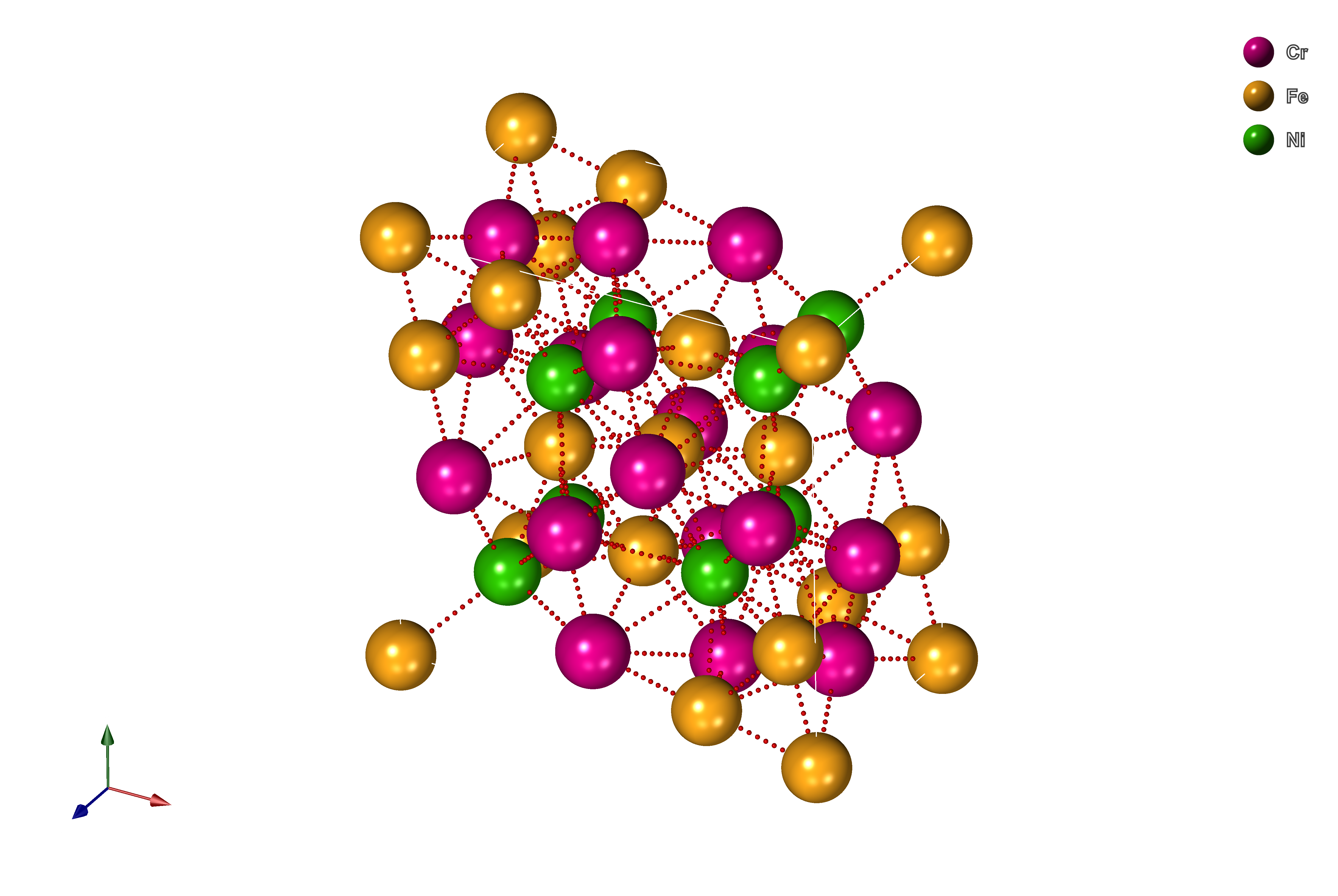
# More Complex Structures
Armed with all the basics, let's look at some more complex structures and start to modify them! For that purpose, we will take a topologically close-packed (TCP) phase from the Cr-Fe-Ni system called Sigma, which is both difficult to predict and critical to the performance of Ni-based superalloys.
The structure is available here under assets/0-Cr8Fe18Ni4.POSCAR, in plain-text looking like
Cr8 Fe18 Ni4
1.0
8.547048 0.000000 0.000000
0.000000 8.547048 0.000000
0.000000 0.000000 4.477714
Cr Fe Ni
8 18 4
direct
0.737702 0.063709 0.000000 Cr
0.262298 0.936291 0.000000 Cr
...
0.899910 0.100090 0.500000 Ni
,or when visualized:
Now, we can quickly load it into pymatgen with either (1) Structure.from_file or (2) pymatgen.io.vasp module using Poscar class, with the latter being more reliable in some cases. Since it is an example of Sigma TCP phase occupation, we will call it baseStructure.
baseStructure = Structure.from_file("assets/0-Cr8Fe18Ni4.POSCAR")
baseStructure
Structure Summary
Lattice
    abc : 8.547048 8.547048 4.477714
 angles : 90.0 90.0 90.0
 volume : 327.10609528461225
      A : 8.547048 0.0 0.0
      B : 0.0 8.547048 0.0
      C : 0.0 0.0 4.477714
    pbc : True True True
PeriodicSite: Cr (6.305, 0.5445, 0.0) [0.7377, 0.06371, 0.0]
PeriodicSite: Cr (2.242, 8.003, 0.0) [0.2623, 0.9363, 0.0]
PeriodicSite: Cr (3.729, 2.032, 2.239) [0.4363, 0.2377, 0.5]
PeriodicSite: Cr (6.515, 4.818, 2.239) [0.7623, 0.5637, 0.5]
PeriodicSite: Cr (4.818, 6.515, 2.239) [0.5637, 0.7623, 0.5]
PeriodicSite: Cr (2.032, 3.729, 2.239) [0.2377, 0.4363, 0.5]
PeriodicSite: Cr (0.5445, 6.305, 0.0) [0.06371, 0.7377, 0.0]
PeriodicSite: Cr (8.003, 2.242, 0.0) [0.9363, 0.2623, 0.0]
PeriodicSite: Fe (0.0, 0.0, 0.0) [0.0, 0.0, 0.0]
PeriodicSite: Fe (4.274, 4.274, 2.239) [0.5, 0.5, 0.5]
PeriodicSite: Fe (3.958, 1.107, 0.0) [0.463, 0.1295, 0.0]
PeriodicSite: Fe (4.59, 7.44, 0.0) [0.537, 0.8705, 0.0]
PeriodicSite: Fe (3.167, 8.231, 2.239) [0.3705, 0.963, 0.5]
PeriodicSite: Fe (0.316, 5.38, 2.239) [0.03697, 0.6295, 0.5]
PeriodicSite: Fe (5.38, 0.316, 2.239) [0.6295, 0.03697, 0.5]
PeriodicSite: Fe (8.231, 3.167, 2.239) [0.963, 0.3705, 0.5]
PeriodicSite: Fe (1.107, 3.958, 0.0) [0.1295, 0.463, 0.0]
PeriodicSite: Fe (7.44, 4.59, 0.0) [0.8705, 0.537, 0.0]
PeriodicSite: Fe (1.562, 1.562, 1.127) [0.1827, 0.1827, 0.2517]
PeriodicSite: Fe (6.985, 6.985, 3.351) [0.8173, 0.8173, 0.7483]
PeriodicSite: Fe (6.985, 6.985, 1.127) [0.8173, 0.8173, 0.2517]
PeriodicSite: Fe (2.712, 5.835, 3.366) [0.3173, 0.6827, 0.7517]
PeriodicSite: Fe (2.712, 5.835, 1.112) [0.3173, 0.6827, 0.2483]
PeriodicSite: Fe (1.562, 1.562, 3.351) [0.1827, 0.1827, 0.7483]
PeriodicSite: Fe (5.835, 2.712, 1.112) [0.6827, 0.3173, 0.2483]
PeriodicSite: Fe (5.835, 2.712, 3.366) [0.6827, 0.3173, 0.7517]
PeriodicSite: Ni (3.418, 3.418, 0.0) [0.3999, 0.3999, 0.0]
PeriodicSite: Ni (5.129, 5.129, 0.0) [0.6001, 0.6001, 0.0]
PeriodicSite: Ni (0.8555, 7.692, 2.239) [0.1001, 0.8999, 0.5]
PeriodicSite: Ni (7.692, 0.8555, 2.239) [0.8999, 0.1001, 0.5]
Now, we can quickly investigate the symmetry with tools we just learned:
spgA = SpacegroupAnalyzer(baseStructure)
spgA.get_symmetrized_structure()
SymmetrizedStructure
Full Formula (Cr8 Fe18 Ni4)
Reduced Formula: Cr4Fe9Ni2
Spacegroup: P4_2/mnm (136)
abc   :   8.547048   8.547048   4.477714
angles:  90.000000  90.000000  90.000000
Sites (30)
  #  SP           a         b         c  Wyckoff
---  ----  --------  --------  --------  ---------
  0  Cr    0.737702  0.063709  0         8i
  1  Fe    0         0         0         2a
  2  Fe    0.463029  0.129472  0         8i
  3  Fe    0.182718  0.182718  0.251726  8j
  4  Ni    0.39991   0.39991   0         4f
We can quickly see that our atomic configuration has 5 chemically unique sites of different multiplicities occupied by the 3 elements of interest. However, performing the analysis like that can quickly lead to problems if, for instance, we introduce even a tiny disorder in the structure, like a substitutional defect.
sDilute = copy(baseStructure)
sDilute.replace(0, "Fe")
spgA = SpacegroupAnalyzer(sDilute)
spgA.get_symmetrized_structure()
SymmetrizedStructure
Full Formula (Cr7 Fe19 Ni4)
Reduced Formula: Cr7Fe19Ni4
Spacegroup: Pm (6)
abc   :   8.547048   8.547048   4.477714
angles:  90.000000  90.000000  90.000000
Sites (30)
  #  SP           a         b         c  Wyckoff
---  ----  --------  --------  --------  ---------
  0  Fe    0.737702  0.063709  0         1a
  1  Cr    0.262298  0.936291  0         1a
  2  Cr    0.436291  0.237702  0.5       1b
  3  Cr    0.762298  0.563709  0.5       1b
  4  Cr    0.563709  0.762298  0.5       1b
  5  Cr    0.237702  0.436291  0.5       1b
  6  Cr    0.063709  0.737702  0         1a
  7  Cr    0.936291  0.262298  0         1a
  8  Fe    0         0         0         1a
  9  Fe    0.5       0.5       0.5       1b
 10  Fe    0.463029  0.129472  0         1a
 11  Fe    0.536971  0.870528  0         1a
 12  Fe    0.370528  0.963029  0.5       1b
 13  Fe    0.036971  0.629472  0.5       1b
 14  Fe    0.629472  0.036971  0.5       1b
 15  Fe    0.963029  0.370528  0.5       1b
 16  Fe    0.129472  0.463029  0         1a
 17  Fe    0.870528  0.536971  0         1a
 18  Fe    0.182718  0.182718  0.251726  2c
 19  Fe    0.817282  0.817282  0.748274  2c
 20  Fe    0.317282  0.682718  0.751726  2c
 21  Fe    0.682718  0.317282  0.248274  2c
 22  Ni    0.39991   0.39991   0         1a
 23  Ni    0.60009   0.60009   0         1a
 24  Ni    0.10009   0.89991   0.5       1b
 25  Ni    0.89991   0.10009   0.5       1b
Without any change to the other 29 atoms, there are 25 unique sites rather than 5. Thus, if one wants to see what are the symmetry-enforced unique sites, determining underlying sublattices, in the structure, one needs anonymize the atoms first.
for el in set(baseStructure.species):
    baseStructure.replace_species({el: 'dummy'})
print(baseStructure)
Full Formula (Dummy30)
Reduced Formula: Dummy
abc   :   8.547048   8.547048   4.477714
angles:  90.000000  90.000000  90.000000
pbc   :       True       True       True
Sites (30)
  #  SP              a         b         c
---  -------  --------  --------  --------
  0  Dummy0+  0.737702  0.063709  0
  1  Dummy0+  0.262298  0.936291  0
  2  Dummy0+  0.436291  0.237702  0.5
  3  Dummy0+  0.762298  0.563709  0.5
  4  Dummy0+  0.563709  0.762298  0.5
  5  Dummy0+  0.237702  0.436291  0.5
  6  Dummy0+  0.063709  0.737702  0
  7  Dummy0+  0.936291  0.262298  0
  8  Dummy0+  0         0         0
  9  Dummy0+  0.5       0.5       0.5
 10  Dummy0+  0.463029  0.129472  0
 11  Dummy0+  0.536971  0.870528  0
 12  Dummy0+  0.370528  0.963029  0.5
 13  Dummy0+  0.036971  0.629472  0.5
 14  Dummy0+  0.629472  0.036971  0.5
 15  Dummy0+  0.963029  0.370528  0.5
 16  Dummy0+  0.129472  0.463029  0
 17  Dummy0+  0.870528  0.536971  0
 18  Dummy0+  0.182718  0.182718  0.251726
 19  Dummy0+  0.817282  0.817282  0.748274
 20  Dummy0+  0.817282  0.817282  0.251726
 21  Dummy0+  0.317282  0.682718  0.751726
 22  Dummy0+  0.317282  0.682718  0.248274
 23  Dummy0+  0.182718  0.182718  0.748274
 24  Dummy0+  0.682718  0.317282  0.248274
 25  Dummy0+  0.682718  0.317282  0.751726
 26  Dummy0+  0.39991   0.39991   0
 27  Dummy0+  0.60009   0.60009   0
 28  Dummy0+  0.10009   0.89991   0.5
 29  Dummy0+  0.89991   0.10009   0.5
Which we then pass to the SpacegroupAnalyzer to get the symmetry information as before:
spgA = SpacegroupAnalyzer(baseStructure)
spgA.get_symmetrized_structure()
SymmetrizedStructure
Full Formula (Dummy30)
Reduced Formula: Dummy
Spacegroup: P4_2/mnm (136)
abc   :   8.547048   8.547048   4.477714
angles:  90.000000  90.000000  90.000000
Sites (30)
  #  SP              a         b         c  Wyckoff
---  -------  --------  --------  --------  ---------
  0  Dummy0+  0.737702  0.063709  0         8i
  1  Dummy0+  0         0         0         2a
  2  Dummy0+  0.463029  0.129472  0         8i
  3  Dummy0+  0.182718  0.182718  0.251726  8j
  4  Dummy0+  0.39991   0.39991   0         4f
Or we can turn into a useful dict for generating all possible occupancies of the structure.
spgA = SpacegroupAnalyzer(baseStructure)
uniqueDict = defaultdict(list)
for site, unique in enumerate(spgA.get_symmetry_dataset()['equivalent_atoms']):
    uniqueDict[unique] += [site]
pprint(uniqueDict)
defaultdict(<class 'list'>,
            {0: [0, 1, 2, 3, 4, 5, 6, 7],
             8: [8, 9],
             10: [10, 11, 12, 13, 14, 15, 16, 17],
             18: [18, 19, 20, 21, 22, 23, 24, 25],
             26: [26, 27, 28, 29]})
from itertools import product
allPermutations = list(product(['Fe', 'Cr', 'Ni'], repeat=5))
print(f'Obtained {len(allPermutations)} permutations of the sublattice occupancy\nE.g.:  {allPermutations[32]}')
Obtained 243 permutations of the sublattice occupancy
E.g.:  ('Fe', 'Cr', 'Fe', 'Cr', 'Ni')
We can now generate them iteratively, as done below:
structList = []
for permutation in allPermutations:
    tempStructure = baseStructure.copy()
    for unique, el in zip(uniqueDict, permutation):
        for site in uniqueDict[unique]:
            tempStructure.replace(site, el)
    structList.append(tempStructure)
print(structList[25])
Full Formula (Cr4 Fe10 Ni16)
Reduced Formula: Cr2Fe5Ni8
abc   :   8.547048   8.547048   4.477714
angles:  90.000000  90.000000  90.000000
pbc   :       True       True       True
Sites (30)
  #  SP           a         b         c
---  ----  --------  --------  --------
  0  Fe    0.737702  0.063709  0
  1  Fe    0.262298  0.936291  0
  2  Fe    0.436291  0.237702  0.5
  3  Fe    0.762298  0.563709  0.5
  4  Fe    0.563709  0.762298  0.5
  5  Fe    0.237702  0.436291  0.5
  6  Fe    0.063709  0.737702  0
  7  Fe    0.936291  0.262298  0
  8  Fe    0         0         0
  9  Fe    0.5       0.5       0.5
 10  Ni    0.463029  0.129472  0
 11  Ni    0.536971  0.870528  0
 12  Ni    0.370528  0.963029  0.5
 13  Ni    0.036971  0.629472  0.5
 14  Ni    0.629472  0.036971  0.5
 15  Ni    0.963029  0.370528  0.5
 16  Ni    0.129472  0.463029  0
 17  Ni    0.870528  0.536971  0
 18  Ni    0.182718  0.182718  0.251726
 19  Ni    0.817282  0.817282  0.748274
 20  Ni    0.817282  0.817282  0.251726
 21  Ni    0.317282  0.682718  0.751726
 22  Ni    0.317282  0.682718  0.248274
 23  Ni    0.182718  0.182718  0.748274
 24  Ni    0.682718  0.317282  0.248274
 25  Ni    0.682718  0.317282  0.751726
 26  Cr    0.39991   0.39991   0
 27  Cr    0.60009   0.60009   0
 28  Cr    0.10009   0.89991   0.5
 29  Cr    0.89991   0.10009   0.5
# Persisting on Disk
The easiest way to persist a structure on disk is to use the to method of the Structure object, which will write the structure in a variety of formats, including POSCAR and CIF:
os.mkdir('POSCARs')
os.mkdir('CIFs')
for struct, permutation in zip(structList, allPermutations):
    struct.to(filename='POSCARs/' + "".join(permutation) + '.POSCAR')
    struct.to(filename='CIFs/' + "".join(permutation) + '.cif')
And now we are ready to use them in a variety of other tools like DFTTK covered last week or pySIPFENN covered during the next lecture!
# Setting up MongoDB
With the ability to manipulate structures locally, one will quickly run into two major problems:
- How to pass them between personal laptop, HPC clusters, and lab workstations?
- How do I share them with others later?
One of the easiest ways to do so is to use a cloud-based database, which will allow us to synchronize our work regardless of what machine we use and then share it with others in a highly secure way or publicly, as needed. In this lecture, we will use MongoDB Atlas to set up a small NoSQL database on the cloud. For our needs and most of the other personal needs of researchers, the Free Tier will be more than enough, but if you need more, you can always upgrade to a paid plan for a few dollars a month if you need to store tens of thousands of structures.
Note for Online Students: At this point, we will pause the Jupiter Notebook and switch to the MongoDB Atlas website to set up the database. The process is fairly straightforward but feel free to stop by during office hours for help!
Now, we should have the following:
- A database called
matse580with a collection calledstructures - User with read/write access named
student - API key for the user to access the database (looks like
2fnc92niu2bnc9o240dc) - Resulting connection string to the database (looks like
mongodb+srv://student:2fnc92niu2bnc9o240dc@<cluster_name>/matse580) and we can move to populating it with data!
# Pymongo
# Connecting
The pymongo is a Python library that allows us to interact with MongoDB databases in a very intuitive way. Let's start by importing its MongoClient class and creating a connection to our database:
from pymongo import MongoClient
uri = 'mongodb+srv://amk7137:kASMuF5au1069Go8@cluster0.3wlhaan.mongodb.net/?retryWrites=true&w=majority'
client = MongoClient(uri)
We can see what databases are available:
client.list_database_names()
Lets now go back to MongoDB Atlas and create a new database called matse580 and a collection called structures in it, and hopefully see that they are /available:
client.list_database_names()
['matse580', 'admin', 'local']
To go one level deeper and see what collections are available in the matse580 database we just created, we can use the list_collection_names method:
database = client['matse580']
database.list_collection_names()
['structures']
And then read the entries in it!
collection = database['structures']
for entry in collection.find():
    print(entry)
But that's not very useful, because we didn't put anything in it yet.
# Inserting Data
We start by constructing our idea of how a structure should be represented in the database. For that purpose, we will use a dictionary representation of the structure. This process is very flexible as NoSQL databases like MongoDB do not require a strict schema and can be modified on the fly and post-processed later. For our purposes, we will use the following schema:
def struct2entry(s: Structure):
    strcutreDict = {'structure': s.as_dict()} # convert to pymatgen Structure dictionary default
    compositionDict = {'composition': s.composition.as_dict()} # convert to pymatgen Composition dictionary default
    entry = {**strcutreDict, **compositionDict} # merge the two dictionaries
    # add some extra information
    entry.update({'density': s.density,
                  'volume': s.volume,
                  'reducedFormula': s.composition.reduced_formula,
                  'weightFractions': s.composition.to_weight_dict
                  })
    # and a full POSCAR for easy ingestion into VASP
    entry.update({'POSCAR': s.to(fmt='poscar')})
    return entry
pprint(struct2entry(structList[25]))
{'POSCAR': 'Cr4 Fe10 Ni16\n'
'1.0\n'
' 8.5470480000000002 0.0000000000000000 0.0000000000000000\n'
' 0.0000000000000000 8.5470480000000002 0.0000000000000000\n'
' 0.0000000000000000 0.0000000000000000 4.4777139999999997\n'
'Fe Ni Cr\n'
'10 16 4\n'
'direct\n'
' 0.7377020000000000 0.0637090000000000 0.0000000000000000 '
'Fe\n'
' 0.2622980000000000 0.9362910000000000 0.0000000000000000 '
'Fe\n'
' 0.4362910000000000 0.2377020000000000 0.5000000000000000 '
'Fe\n'
' 0.7622980000000000 0.5637090000000000 0.5000000000000000 '
'Fe\n'
' 0.5637090000000000 0.7622980000000000 0.5000000000000000 '
'Fe\n'
' 0.2377020000000000 0.4362910000000000 0.5000000000000000 '
'Fe\n'
' 0.0637090000000000 0.7377020000000000 0.0000000000000000 '
'Fe\n'
' 0.9362910000000000 0.2622980000000000 0.0000000000000000 '
'Fe\n'
' 0.0000000000000000 0.0000000000000000 0.0000000000000000 '
'Fe\n'
' 0.5000000000000000 0.5000000000000000 0.5000000000000000 '
'Fe\n'
' 0.4630290000000000 0.1294720000000000 0.0000000000000000 '
'Ni\n'
' 0.5369710000000000 0.8705280000000000 0.0000000000000000 '
'Ni\n'
' 0.3705280000000000 0.9630290000000000 0.5000000000000000 '
'Ni\n'
' 0.0369710000000000 0.6294720000000000 0.5000000000000000 '
'Ni\n'
' 0.6294720000000000 0.0369710000000000 0.5000000000000000 '
'Ni\n'
' 0.9630290000000000 0.3705280000000000 0.5000000000000000 '
'Ni\n'
' 0.1294720000000000 0.4630290000000000 0.0000000000000000 '
'Ni\n'
' 0.8705280000000000 0.5369710000000000 0.0000000000000000 '
'Ni\n'
' 0.1827180000000000 0.1827180000000000 0.2517260000000000 '
'Ni\n'
' 0.8172820000000000 0.8172820000000000 0.7482740000000000 '
'Ni\n'
' 0.8172820000000000 0.8172820000000000 0.2517260000000000 '
'Ni\n'
' 0.3172820000000000 0.6827180000000000 0.7517260000000000 '
'Ni\n'
' 0.3172820000000000 0.6827180000000000 0.2482740000000000 '
'Ni\n'
' 0.1827180000000000 0.1827180000000000 0.7482740000000000 '
'Ni\n'
' 0.6827180000000000 0.3172820000000000 0.2482740000000000 '
'Ni\n'
' 0.6827180000000000 0.3172820000000000 0.7517260000000000 '
'Ni\n'
' 0.3999100000000000 0.3999100000000000 0.0000000000000000 '
'Cr\n'
' 0.6000900000000000 0.6000900000000000 0.0000000000000000 '
'Cr\n'
' 0.1000900000000000 0.8999100000000000 0.5000000000000000 '
'Cr\n'
' 0.8999100000000000 0.1000900000000000 0.5000000000000000 '
'Cr\n',
'composition': {'Cr': 4.0, 'Fe': 10.0, 'Ni': 16.0},
'density': 8.658038607159655,
'reducedFormula': 'Cr2Fe5Ni8',
'structure': {'@class': 'Structure',
'@module': 'pymatgen.core.structure',
'charge': 0,
'lattice': {'a': 8.547048,
'alpha': 90.0,
'b': 8.547048,
'beta': 90.0,
'c': 4.477714,
'gamma': 90.0,
'matrix': [[8.547048, 0.0, 0.0],
[0.0, 8.547048, 0.0],
[0.0, 0.0, 4.477714]],
'pbc': (True, True, True),
'volume': 327.10609528461225},
'properties': {},
'sites': [{'abc': [0.737702, 0.063709, 0.0],
'label': 'Fe',
'properties': {},
'species': [{'element': 'Fe', 'occu': 1}],
'xyz': [6.305174403696, 0.544523881032, 0.0]},
{'abc': [0.262298, 0.936291, 0.0],
'label': 'Fe',
'properties': {},
'species': [{'element': 'Fe', 'occu': 1}],
'xyz': [2.241873596304, 8.002524118968, 0.0]},
{'abc': [0.436291, 0.237702, 0.5],
'label': 'Fe',
'properties': {},
'species': [{'element': 'Fe', 'occu': 1}],
'xyz': [3.729000118968, 2.031650403696, 2.238857]},
{'abc': [0.762298, 0.563709, 0.5],
'label': 'Fe',
'properties': {},
'species': [{'element': 'Fe', 'occu': 1}],
'xyz': [6.515397596304, 4.818047881032, 2.238857]},
{'abc': [0.563709, 0.762298, 0.5],
'label': 'Fe',
'properties': {},
'species': [{'element': 'Fe', 'occu': 1}],
'xyz': [4.818047881032, 6.515397596304, 2.238857]},
{'abc': [0.237702, 0.436291, 0.5],
'label': 'Fe',
'properties': {},
'species': [{'element': 'Fe', 'occu': 1}],
'xyz': [2.031650403696, 3.729000118968, 2.238857]},
{'abc': [0.063709, 0.737702, 0.0],
'label': 'Fe',
'properties': {},
'species': [{'element': 'Fe', 'occu': 1}],
'xyz': [0.544523881032, 6.305174403696, 0.0]},
{'abc': [0.936291, 0.262298, 0.0],
'label': 'Fe',
'properties': {},
'species': [{'element': 'Fe', 'occu': 1}],
'xyz': [8.002524118968, 2.241873596304, 0.0]},
{'abc': [0.0, 0.0, 0.0],
'label': 'Fe',
'properties': {},
'species': [{'element': 'Fe', 'occu': 1}],
'xyz': [0.0, 0.0, 0.0]},
{'abc': [0.5, 0.5, 0.5],
'label': 'Fe',
'properties': {},
'species': [{'element': 'Fe', 'occu': 1}],
'xyz': [4.273524, 4.273524, 2.238857]},
{'abc': [0.463029, 0.129472, 0.0],
'label': 'Ni',
'properties': {},
'species': [{'element': 'Ni', 'occu': 1}],
'xyz': [3.9575310883920003, 1.106603398656, 0.0]},
{'abc': [0.536971, 0.870528, 0.0],
'label': 'Ni',
'properties': {},
'species': [{'element': 'Ni', 'occu': 1}],
'xyz': [4.5895169116079995, 7.440444601344, 0.0]},
{'abc': [0.370528, 0.963029, 0.5],
'label': 'Ni',
'properties': {},
'species': [{'element': 'Ni', 'occu': 1}],
'xyz': [3.166920601344, 8.231055088392, 2.238857]},
{'abc': [0.036971, 0.629472, 0.5],
'label': 'Ni',
'properties': {},
'species': [{'element': 'Ni', 'occu': 1}],
'xyz': [0.31599291160799997,
5.3801273986560005,
2.238857]},
{'abc': [0.629472, 0.036971, 0.5],
'label': 'Ni',
'properties': {},
'species': [{'element': 'Ni', 'occu': 1}],
'xyz': [5.3801273986560005,
0.31599291160799997,
2.238857]},
{'abc': [0.963029, 0.370528, 0.5],
'label': 'Ni',
'properties': {},
'species': [{'element': 'Ni', 'occu': 1}],
'xyz': [8.231055088392, 3.166920601344, 2.238857]},
{'abc': [0.129472, 0.463029, 0.0],
'label': 'Ni',
'properties': {},
'species': [{'element': 'Ni', 'occu': 1}],
'xyz': [1.106603398656, 3.9575310883920003, 0.0]},
{'abc': [0.870528, 0.536971, 0.0],
'label': 'Ni',
'properties': {},
'species': [{'element': 'Ni', 'occu': 1}],
'xyz': [7.440444601344, 4.5895169116079995, 0.0]},
{'abc': [0.182718, 0.182718, 0.251726],
'label': 'Ni',
'properties': {},
'species': [{'element': 'Ni', 'occu': 1}],
'xyz': [1.561699516464,
1.561699516464,
1.127157034364]},
{'abc': [0.817282, 0.817282, 0.748274],
'label': 'Ni',
'properties': {},
'species': [{'element': 'Ni', 'occu': 1}],
'xyz': [6.985348483536,
6.985348483536,
3.3505569656359997]},
{'abc': [0.817282, 0.817282, 0.251726],
'label': 'Ni',
'properties': {},
'species': [{'element': 'Ni', 'occu': 1}],
'xyz': [6.985348483536,
6.985348483536,
1.127157034364]},
{'abc': [0.317282, 0.682718, 0.751726],
'label': 'Ni',
'properties': {},
'species': [{'element': 'Ni', 'occu': 1}],
'xyz': [2.711824483536,
5.8352235164640005,
3.366014034364]},
{'abc': [0.317282, 0.682718, 0.248274],
'label': 'Ni',
'properties': {},
'species': [{'element': 'Ni', 'occu': 1}],
'xyz': [2.711824483536,
5.8352235164640005,
1.1116999656359998]},
{'abc': [0.182718, 0.182718, 0.748274],
'label': 'Ni',
'properties': {},
'species': [{'element': 'Ni', 'occu': 1}],
'xyz': [1.561699516464,
1.561699516464,
3.3505569656359997]},
{'abc': [0.682718, 0.317282, 0.248274],
'label': 'Ni',
'properties': {},
'species': [{'element': 'Ni', 'occu': 1}],
'xyz': [5.8352235164640005,
2.711824483536,
1.1116999656359998]},
{'abc': [0.682718, 0.317282, 0.751726],
'label': 'Ni',
'properties': {},
'species': [{'element': 'Ni', 'occu': 1}],
'xyz': [5.8352235164640005,
2.711824483536,
3.366014034364]},
{'abc': [0.39991, 0.39991, 0.0],
'label': 'Cr',
'properties': {},
'species': [{'element': 'Cr', 'occu': 1}],
'xyz': [3.41804996568, 3.41804996568, 0.0]},
{'abc': [0.60009, 0.60009, 0.0],
'label': 'Cr',
'properties': {},
'species': [{'element': 'Cr', 'occu': 1}],
'xyz': [5.12899803432, 5.12899803432, 0.0]},
{'abc': [0.10009, 0.89991, 0.5],
'label': 'Cr',
'properties': {},
'species': [{'element': 'Cr', 'occu': 1}],
'xyz': [0.85547403432, 7.69157396568, 2.238857]},
{'abc': [0.89991, 0.10009, 0.5],
'label': 'Cr',
'properties': {},
'species': [{'element': 'Cr', 'occu': 1}],
'xyz': [7.69157396568, 0.85547403432, 2.238857]}]},
'volume': 327.10609528461225,
'weightFractions': {'Cr': 0.12194716383563854,
'Fe': 0.3274351039982438,
'Ni': 0.5506177321661175}}
Looks great! Now we can add some metadata to it, like who created it, when, and what was the permutation label used to generate it earlier; to then insert it into the database using the insert_one method, which is not the fastest, but the most flexible way to do so:
for struct, permutation in zip(structList, allPermutations):
    entry = struct2entry(struct)
    entry.update({'permutation': "".join(permutation),
                  'autor': 'Happy Student',
                  'creationDate': datetime.now(ZoneInfo('America/New_York'))
                })
    collection.insert_one(entry)
We can now quickly check if they are present by counting the number of entries in the collection:
collection.count_documents({})
243
If something went wrong halfway, you can start over by deleting all entries in the collection (be careful with this one!):
# Uncomment to run
#collection.delete_many({})
#collection.count_documents({})
# Updating Data
This will be reiterated in the next lecture, but in principle updating the data is easy. For example, we can add a new field to the document, like averageElectronegativity by iterating over all entries present in the collection and calculating it:
for entry in collection.find():
    id = entry['_id']
    s = Structure.from_dict(entry['structure'])
    collection.update_one({'_id': id}, {'$set': {'averageElectronegativity': s.composition.average_electroneg}})
Or, to remove a field, like volume, which happens to be the same for all structures, we can do it in a similar way:
for entry in collection.find():
    id = entry['_id']
    collection.update_one({'_id': id}, {'$unset': {'volume': ''}})
Since we apply it in the same way on all entries, we can do it in a single line of code using the update_many method and an empty filter {} querying all entries:
collection.update_many({}, {'$unset': {'volume': ''}})
<pymongo.results.UpdateResult at 0x294323340>
# Querying Data
Now that we have some data in the database, we can start querying it. MongoDB has state-of-the-art query language that allows us to do very complex queries and do them with extreme performance. You can find more information about it in this documentation but for our purposes, we will stick to the basics like finding all Cr-containing structures.
To find all entries in the collection, we can use the find method with a dictionary of query parameters. We can use many different methods, but the simplest would be to look for a composition dictionary with over-0 or non-empty values for Cr:
for entry in collection.find({'weightFractions.Cr': {'$gt': 0}}):
    print(entry['reducedFormula'])
Cr2Fe13
Cr4Fe11
Cr2Fe3
Cr4Fe9Ni2
Cr2Fe9Ni4
Cr4Fe11
Cr2Fe3
Cr4Fe9Ni2
Cr8Fe7
Cr2Fe
Cr8Fe5Ni2
Cr4Fe7Ni4
Cr6Fe5Ni4
Cr4Fe5Ni6
Cr2Fe9Ni4
Cr4Fe7Ni4
Cr6Fe5Ni4
Cr4Fe5Ni6
Cr2Fe5Ni8
CrFe14
CrFe4
Cr(Fe6Ni)2
CrFe2
Cr7Fe8
Cr5(Fe4Ni)2
Cr(Fe5Ni2)2
Cr3(Fe2Ni)4
Cr(Fe4Ni3)2
CrFe2
Cr7Fe8
Cr5(Fe4Ni)2
Cr3Fe2
Cr11Fe4
Cr9(Fe2Ni)2
Cr5(Fe3Ni2)2
Cr7(FeNi)4
Cr5(Fe2Ni3)2
Cr(Fe5Ni2)2
Cr3(Fe2Ni)4
Cr(Fe4Ni3)2
Cr5(Fe3Ni2)2
Cr7(FeNi)4
Cr5(Fe2Ni3)2
Cr(Fe3Ni4)2
Cr3(FeNi2)4
Cr(Fe2Ni5)2
Cr2Fe12Ni
Cr4Fe10Ni
Cr6Fe8Ni
Cr4Fe8Ni3
Cr2Fe8Ni5
Cr4Fe10Ni
Cr6Fe8Ni
Cr4Fe8Ni3
Cr8Fe6Ni
Cr10Fe4Ni
Cr8Fe4Ni3
Cr4Fe6Ni5
Cr6Fe4Ni5
Cr4Fe4Ni7
Cr2Fe8Ni5
Cr4Fe6Ni5
Cr6Fe4Ni5
Cr4Fe4Ni7
Cr2Fe4Ni9
Cr4Fe11
Cr2Fe3
Cr4Fe9Ni2
Cr8Fe7
Cr2Fe
Cr8Fe5Ni2
Cr4Fe7Ni4
Cr6Fe5Ni4
Cr4Fe5Ni6
Cr8Fe7
Cr2Fe
Cr8Fe5Ni2
Cr4Fe
Cr14Fe
Cr12FeNi2
Cr8Fe3Ni4
Cr10FeNi4
Cr8FeNi6
Cr4Fe7Ni4
Cr6Fe5Ni4
Cr4Fe5Ni6
Cr8Fe3Ni4
Cr10FeNi4
Cr8FeNi6
Cr4Fe3Ni8
Cr6FeNi8
Cr4FeNi10
CrFe2
Cr7Fe8
Cr5(Fe4Ni)2
Cr3Fe2
Cr11Fe4
Cr9(Fe2Ni)2
Cr5(Fe3Ni2)2
Cr7(FeNi)4
Cr5(Fe2Ni3)2
Cr3Fe2
Cr11Fe4
Cr9(Fe2Ni)2
Cr13Fe2
Cr
Cr13Ni2
Cr9(FeNi2)2
Cr11Ni4
Cr3Ni2
Cr5(Fe3Ni2)2
Cr7(FeNi)4
Cr5(Fe2Ni3)2
Cr9(FeNi2)2
Cr11Ni4
Cr3Ni2
Cr5(FeNi4)2
Cr7Ni8
CrNi2
Cr4Fe10Ni
Cr6Fe8Ni
Cr4Fe8Ni3
Cr8Fe6Ni
Cr10Fe4Ni
Cr8Fe4Ni3
Cr4Fe6Ni5
Cr6Fe4Ni5
Cr4Fe4Ni7
Cr8Fe6Ni
Cr10Fe4Ni
Cr8Fe4Ni3
Cr12Fe2Ni
Cr14Ni
Cr4Ni
Cr8Fe2Ni5
Cr2Ni
Cr8Ni7
Cr4Fe6Ni5
Cr6Fe4Ni5
Cr4Fe4Ni7
Cr8Fe2Ni5
Cr2Ni
Cr8Ni7
Cr4Fe2Ni9
Cr2Ni3
Cr4Ni11
Cr2Fe9Ni4
Cr4Fe7Ni4
Cr6Fe5Ni4
Cr4Fe5Ni6
Cr2Fe5Ni8
Cr4Fe7Ni4
Cr6Fe5Ni4
Cr4Fe5Ni6
Cr8Fe3Ni4
Cr10FeNi4
Cr8FeNi6
Cr4Fe3Ni8
Cr6FeNi8
Cr4FeNi10
Cr2Fe5Ni8
Cr4Fe3Ni8
Cr6FeNi8
Cr4FeNi10
Cr2FeNi12
Cr(Fe5Ni2)2
Cr3(Fe2Ni)4
Cr(Fe4Ni3)2
Cr5(Fe3Ni2)2
Cr7(FeNi)4
Cr5(Fe2Ni3)2
Cr(Fe3Ni4)2
Cr3(FeNi2)4
Cr(Fe2Ni5)2
Cr5(Fe3Ni2)2
Cr7(FeNi)4
Cr5(Fe2Ni3)2
Cr9(FeNi2)2
Cr11Ni4
Cr3Ni2
Cr5(FeNi4)2
Cr7Ni8
CrNi2
Cr(Fe3Ni4)2
Cr3(FeNi2)4
Cr(Fe2Ni5)2
Cr5(FeNi4)2
Cr7Ni8
CrNi2
Cr(FeNi6)2
CrNi4
CrNi14
Cr2Fe8Ni5
Cr4Fe6Ni5
Cr6Fe4Ni5
Cr4Fe4Ni7
Cr2Fe4Ni9
Cr4Fe6Ni5
Cr6Fe4Ni5
Cr4Fe4Ni7
Cr8Fe2Ni5
Cr2Ni
Cr8Ni7
Cr4Fe2Ni9
Cr2Ni3
Cr4Ni11
Cr2Fe4Ni9
Cr4Fe2Ni9
Cr2Ni3
Cr4Ni11
Cr2Ni13
for entry in collection.find({'weightFractions.Cr': {'$ne': None}}):
    print(entry['reducedFormula'])
Cr2Fe13
Cr4Fe11
Cr2Fe3
Cr4Fe9Ni2
Cr2Fe9Ni4
Cr4Fe11
Cr2Fe3
Cr4Fe9Ni2
Cr8Fe7
Cr2Fe
Cr8Fe5Ni2
Cr4Fe7Ni4
Cr6Fe5Ni4
Cr4Fe5Ni6
Cr2Fe9Ni4
Cr4Fe7Ni4
Cr6Fe5Ni4
Cr4Fe5Ni6
Cr2Fe5Ni8
CrFe14
CrFe4
Cr(Fe6Ni)2
CrFe2
Cr7Fe8
Cr5(Fe4Ni)2
Cr(Fe5Ni2)2
Cr3(Fe2Ni)4
Cr(Fe4Ni3)2
CrFe2
Cr7Fe8
Cr5(Fe4Ni)2
Cr3Fe2
Cr11Fe4
Cr9(Fe2Ni)2
Cr5(Fe3Ni2)2
Cr7(FeNi)4
Cr5(Fe2Ni3)2
Cr(Fe5Ni2)2
Cr3(Fe2Ni)4
Cr(Fe4Ni3)2
Cr5(Fe3Ni2)2
Cr7(FeNi)4
Cr5(Fe2Ni3)2
Cr(Fe3Ni4)2
Cr3(FeNi2)4
Cr(Fe2Ni5)2
Cr2Fe12Ni
Cr4Fe10Ni
Cr6Fe8Ni
Cr4Fe8Ni3
Cr2Fe8Ni5
Cr4Fe10Ni
Cr6Fe8Ni
Cr4Fe8Ni3
Cr8Fe6Ni
Cr10Fe4Ni
Cr8Fe4Ni3
Cr4Fe6Ni5
Cr6Fe4Ni5
Cr4Fe4Ni7
Cr2Fe8Ni5
Cr4Fe6Ni5
Cr6Fe4Ni5
Cr4Fe4Ni7
Cr2Fe4Ni9
Cr4Fe11
Cr2Fe3
Cr4Fe9Ni2
Cr8Fe7
Cr2Fe
Cr8Fe5Ni2
Cr4Fe7Ni4
Cr6Fe5Ni4
Cr4Fe5Ni6
Cr8Fe7
Cr2Fe
Cr8Fe5Ni2
Cr4Fe
Cr14Fe
Cr12FeNi2
Cr8Fe3Ni4
Cr10FeNi4
Cr8FeNi6
Cr4Fe7Ni4
Cr6Fe5Ni4
Cr4Fe5Ni6
Cr8Fe3Ni4
Cr10FeNi4
Cr8FeNi6
Cr4Fe3Ni8
Cr6FeNi8
Cr4FeNi10
CrFe2
Cr7Fe8
Cr5(Fe4Ni)2
Cr3Fe2
Cr11Fe4
Cr9(Fe2Ni)2
Cr5(Fe3Ni2)2
Cr7(FeNi)4
Cr5(Fe2Ni3)2
Cr3Fe2
Cr11Fe4
Cr9(Fe2Ni)2
Cr13Fe2
Cr
Cr13Ni2
Cr9(FeNi2)2
Cr11Ni4
Cr3Ni2
Cr5(Fe3Ni2)2
Cr7(FeNi)4
Cr5(Fe2Ni3)2
Cr9(FeNi2)2
Cr11Ni4
Cr3Ni2
Cr5(FeNi4)2
Cr7Ni8
CrNi2
Cr4Fe10Ni
Cr6Fe8Ni
Cr4Fe8Ni3
Cr8Fe6Ni
Cr10Fe4Ni
Cr8Fe4Ni3
Cr4Fe6Ni5
Cr6Fe4Ni5
Cr4Fe4Ni7
Cr8Fe6Ni
Cr10Fe4Ni
Cr8Fe4Ni3
Cr12Fe2Ni
Cr14Ni
Cr4Ni
Cr8Fe2Ni5
Cr2Ni
Cr8Ni7
Cr4Fe6Ni5
Cr6Fe4Ni5
Cr4Fe4Ni7
Cr8Fe2Ni5
Cr2Ni
Cr8Ni7
Cr4Fe2Ni9
Cr2Ni3
Cr4Ni11
Cr2Fe9Ni4
Cr4Fe7Ni4
Cr6Fe5Ni4
Cr4Fe5Ni6
Cr2Fe5Ni8
Cr4Fe7Ni4
Cr6Fe5Ni4
Cr4Fe5Ni6
Cr8Fe3Ni4
Cr10FeNi4
Cr8FeNi6
Cr4Fe3Ni8
Cr6FeNi8
Cr4FeNi10
Cr2Fe5Ni8
Cr4Fe3Ni8
Cr6FeNi8
Cr4FeNi10
Cr2FeNi12
Cr(Fe5Ni2)2
Cr3(Fe2Ni)4
Cr(Fe4Ni3)2
Cr5(Fe3Ni2)2
Cr7(FeNi)4
Cr5(Fe2Ni3)2
Cr(Fe3Ni4)2
Cr3(FeNi2)4
Cr(Fe2Ni5)2
Cr5(Fe3Ni2)2
Cr7(FeNi)4
Cr5(Fe2Ni3)2
Cr9(FeNi2)2
Cr11Ni4
Cr3Ni2
Cr5(FeNi4)2
Cr7Ni8
CrNi2
Cr(Fe3Ni4)2
Cr3(FeNi2)4
Cr(Fe2Ni5)2
Cr5(FeNi4)2
Cr7Ni8
CrNi2
Cr(FeNi6)2
CrNi4
CrNi14
Cr2Fe8Ni5
Cr4Fe6Ni5
Cr6Fe4Ni5
Cr4Fe4Ni7
Cr2Fe4Ni9
Cr4Fe6Ni5
Cr6Fe4Ni5
Cr4Fe4Ni7
Cr8Fe2Ni5
Cr2Ni
Cr8Ni7
Cr4Fe2Ni9
Cr2Ni3
Cr4Ni11
Cr2Fe4Ni9
Cr4Fe2Ni9
Cr2Ni3
Cr4Ni11
Cr2Ni13
Or to get a specific permutation, we can use find_one method, which will return the first entry matching the query:
originalStruct25 = collection.find_one({'permutation': 'FeFeNiNiCr'})
originalStruct25['reducedFormula']
'Cr2Fe5Ni8'
# pySIPFENN Install
The last quick thing we will do today is to install pySIPFENN, which is a Python framework which, among other things, allows us to quickly predict stability of materials using machine learning. It can be installed using pip just like pymatgen:
#!pip install pysipfenn
The reason we are installing it here is that the employed models are fairly large and may take a while to download, unless you use cloud virtual machine like GitHub Codespaces. Thus, we will start it now so that it is ready for next week's lecture. Process is automated and you just need to initialize an empty Calculator object:
from pysipfenn import Calculator
c = Calculator()
*********  Initializing pySIPFENN Calculator  **********
Loading model definitions from: /Users/adam/opt/anaconda3/envs/580demo/lib/python3.10/site-packages/pysipfenn/modelsSIPFENN/models.json
Found 4 network definitions in models.json
✔ SIPFENN_Krajewski2020 Standard Materials Model
✔ SIPFENN_Krajewski2020 Novel Materials Model
✔ SIPFENN_Krajewski2020 Light Model
✔ SIPFENN_Krajewski2022 KS2022 Novel Materials Model
Loading all available models (autoLoad=True)
Loading models:


100%|██████████| 4/4 [00:14<00:00,  3.63s/it]

*********  pySIPFENN Successfully Initialized  **********
And then, order it to download the models:
c.downloadModels()
Fetching all networks!
SIPFENN_Krajewski2020_NN9 detected on disk. Ready to use.
SIPFENN_Krajewski2020_NN20 detected on disk. Ready to use.
SIPFENN_Krajewski2020_NN24 detected on disk. Ready to use.
SIPFENN_Krajewski2022_NN30 detected on disk. Ready to use.
All networks available!
✔ SIPFENN_Krajewski2020 Standard Materials Model
✔ SIPFENN_Krajewski2020 Novel Materials Model
✔ SIPFENN_Krajewski2020 Light Model
✔ SIPFENN_Krajewski2022 KS2022 Novel Materials Model
It should take 1-30 minutes depending on your internet connection, but once it is done they will be available until the package is uninstalled. Also, you can run this command as many times as you want, and it will only download the models that are not yet present on your system.