| Main Page | Lecture 1 (native render) | Lecture 2 (native render) |
# Introduction
In this guest lecture, we will cover:
- Interacting with the database we set up in Lecture 1 and visualizing the results - using pymongo library and MongoDB Charts service
- Using machine learning (ML) tools to predict the stability of materials - using pySIPFENN
- Using ML featurization and dimensionality reduction to embed materials in feature space - using pySIPFENN with MongoDB Charts visualization
- Using featurization to guide DFT and improve ML models
This notebook assumes that you already followed the instructions in Lecture 1 and that you:
-
Have a conda environment called
580demo(or other) with all the packages installed, including:pymatgenpymongopysipfenn
-
Have a MongoDB database called
matse580with collectionstructuresto which you have access:- username (e.g.
student) - API key / password string (e.g.
sk39mIM2f35Iwc) - whitelisted your IP address or
0.0.0.0/0(entire internet) - know the connection string (URI) to the database (e.g.
mongodb+srv://student:sk39mIM2f35Iwc@cluster0.3wlhaan.mongodb.net/?retryWrites=true&w=majority)
- username (e.g.
-
You populated the database with all Sigma phase end members (see Lecture 1 - Inserting Data)
-
After you installed
pysipfenn, you have downloaded all the pre-trained models by callingdownloadModels()and it finished successfully. If not, run this one liner:python -c "import pysipfenn; c = pysipfenn.Calculator(); c.downloadModels(); c.loadModels();"
If all of the above are true, you are ready to go!
from pprint import pprint            # pretty printing
from collections import defaultdict  # convenience in the example
import os                            # file handling
from datetime import datetime        # time handling
from zoneinfo import ZoneInfo        # time handling
from pymatgen.core import Structure  # pymatgen
import numpy as np                   # numpy for data manipulation
import plotly.express as px          # plotly for plotting
from importlib import resources      # for accessing the data files
# Verify the connection to the database
As shown in the Lecture 1, pymongo Python library allows us to interact with MongoDB databases in a very intuitive way. Let's start by importing its MongoClient class and creating a connection to our database we have set up.
from pymongo import MongoClient
uri = 'mongodb+srv://amk7137:kASMuF5au1069Go8@cluster0.3wlhaan.mongodb.net/?retryWrites=true&w=majority'
client = MongoClient(uri)
And see what databases are available. If you followed the instructions in Lecture 1, you should see matse580 database in the list.
client.list_database_names()
['matse580', 'admin', 'local']
Now connect to matse580\structures collection
collection = client['matse580']['structures']
And verify that the Sigma phase structures we created are present.
print(f'Found: {collection.count_documents({})} structures\n')
pprint(collection.find_one({}, skip=100))
Found: 243 structures
{'DFT_dH': 0.103503167,
'POSCAR': 'Cr12 Fe10 Ni8\n'
'1.0\n'
' 8.5470480000000002 0.0000000000000000 0.0000000000000000\n'
' 0.0000000000000000 8.5470480000000002 0.0000000000000000\n'
' 0.0000000000000000 0.0000000000000000 4.4777139999999997\n'
'Cr Fe Ni Fe Cr\n'
'8 2 8 8 4\n'
'direct\n'
' 0.7377020000000000 0.0637090000000000 0.0000000000000000 '
'Cr\n'
' 0.2622980000000000 0.9362910000000000 0.0000000000000000 '
'Cr\n'
' 0.4362910000000000 0.2377020000000000 0.5000000000000000 '
'Cr\n'
' 0.7622980000000000 0.5637090000000000 0.5000000000000000 '
'Cr\n'
' 0.5637090000000000 0.7622980000000000 0.5000000000000000 '
'Cr\n'
' 0.2377020000000000 0.4362910000000000 0.5000000000000000 '
'Cr\n'
' 0.0637090000000000 0.7377020000000000 0.0000000000000000 '
'Cr\n'
' 0.9362910000000000 0.2622980000000000 0.0000000000000000 '
'Cr\n'
' 0.0000000000000000 0.0000000000000000 0.0000000000000000 '
'Fe\n'
' 0.5000000000000000 0.5000000000000000 0.5000000000000000 '
'Fe\n'
' 0.4630290000000000 0.1294720000000000 0.0000000000000000 '
'Ni\n'
' 0.5369710000000000 0.8705280000000000 0.0000000000000000 '
'Ni\n'
' 0.3705280000000000 0.9630290000000000 0.5000000000000000 '
'Ni\n'
' 0.0369710000000000 0.6294720000000000 0.5000000000000000 '
'Ni\n'
' 0.6294720000000000 0.0369710000000000 0.5000000000000000 '
'Ni\n'
' 0.9630290000000000 0.3705280000000000 0.5000000000000000 '
'Ni\n'
' 0.1294720000000000 0.4630290000000000 0.0000000000000000 '
'Ni\n'
' 0.8705280000000000 0.5369710000000000 0.0000000000000000 '
'Ni\n'
' 0.1827180000000000 0.1827180000000000 0.2517260000000000 '
'Fe\n'
' 0.8172820000000000 0.8172820000000000 0.7482740000000000 '
'Fe\n'
' 0.8172820000000000 0.8172820000000000 0.2517260000000000 '
'Fe\n'
' 0.3172820000000000 0.6827180000000000 0.7517260000000000 '
'Fe\n'
' 0.3172820000000000 0.6827180000000000 0.2482740000000000 '
'Fe\n'
' 0.1827180000000000 0.1827180000000000 0.7482740000000000 '
'Fe\n'
' 0.6827180000000000 0.3172820000000000 0.2482740000000000 '
'Fe\n'
' 0.6827180000000000 0.3172820000000000 0.7517260000000000 '
'Fe\n'
' 0.3999100000000000 0.3999100000000000 0.0000000000000000 '
'Cr\n'
' 0.6000900000000000 0.6000900000000000 0.0000000000000000 '
'Cr\n'
' 0.1000900000000000 0.8999100000000000 0.5000000000000000 '
'Cr\n'
' 0.8999100000000000 0.1000900000000000 0.5000000000000000 '
'Cr\n',
'SIPFENN_Krajewski2020_NN20': 0.1178784966468811,
'SIPFENN_Krajewski2020_NN24': 0.11623784899711609,
'SIPFENN_Krajewski2020_NN9': 0.15312525629997253,
'TSNE_2D_X': 22.739927291870117,
'TSNE_2D_Y': 63.28989028930664,
'_id': ObjectId('6531516032703fc61d08d457'),
'autor': 'Happy Student',
'averageElectronegativity': 1.7833333333333334,
'composition': {'Cr': 12.0, 'Fe': 10.0, 'Ni': 8.0},
'creationDate': datetime.datetime(2023, 10, 19, 15, 55, 12, 965000),
'density': 8.38605032076435,
'permutation': 'CrFeNiFeCr',
'reducedFormula': 'Cr6Fe5Ni4',
'structure': {'@class': 'Structure',
'@module': 'pymatgen.core.structure',
'charge': 0,
'lattice': {'a': 8.547048,
'alpha': 90.0,
'b': 8.547048,
'beta': 90.0,
'c': 4.477714,
'gamma': 90.0,
'matrix': [[8.547048, 0.0, 0.0],
[0.0, 8.547048, 0.0],
[0.0, 0.0, 4.477714]],
'pbc': [True, True, True],
'volume': 327.10609528461225},
'properties': {},
'sites': [{'abc': [0.737702, 0.063709, 0.0],
'label': 'Cr',
'properties': {},
'species': [{'element': 'Cr', 'occu': 1}],
'xyz': [6.305174403696, 0.544523881032, 0.0]},
{'abc': [0.262298, 0.936291, 0.0],
'label': 'Cr',
'properties': {},
'species': [{'element': 'Cr', 'occu': 1}],
'xyz': [2.241873596304, 8.002524118968, 0.0]},
{'abc': [0.436291, 0.237702, 0.5],
'label': 'Cr',
'properties': {},
'species': [{'element': 'Cr', 'occu': 1}],
'xyz': [3.729000118968, 2.031650403696, 2.238857]},
{'abc': [0.762298, 0.563709, 0.5],
'label': 'Cr',
'properties': {},
'species': [{'element': 'Cr', 'occu': 1}],
'xyz': [6.515397596304, 4.818047881032, 2.238857]},
{'abc': [0.563709, 0.762298, 0.5],
'label': 'Cr',
'properties': {},
'species': [{'element': 'Cr', 'occu': 1}],
'xyz': [4.818047881032, 6.515397596304, 2.238857]},
{'abc': [0.237702, 0.436291, 0.5],
'label': 'Cr',
'properties': {},
'species': [{'element': 'Cr', 'occu': 1}],
'xyz': [2.031650403696, 3.729000118968, 2.238857]},
{'abc': [0.063709, 0.737702, 0.0],
'label': 'Cr',
'properties': {},
'species': [{'element': 'Cr', 'occu': 1}],
'xyz': [0.544523881032, 6.305174403696, 0.0]},
{'abc': [0.936291, 0.262298, 0.0],
'label': 'Cr',
'properties': {},
'species': [{'element': 'Cr', 'occu': 1}],
'xyz': [8.002524118968, 2.241873596304, 0.0]},
{'abc': [0.0, 0.0, 0.0],
'label': 'Fe',
'properties': {},
'species': [{'element': 'Fe', 'occu': 1}],
'xyz': [0.0, 0.0, 0.0]},
{'abc': [0.5, 0.5, 0.5],
'label': 'Fe',
'properties': {},
'species': [{'element': 'Fe', 'occu': 1}],
'xyz': [4.273524, 4.273524, 2.238857]},
{'abc': [0.463029, 0.129472, 0.0],
'label': 'Ni',
'properties': {},
'species': [{'element': 'Ni', 'occu': 1}],
'xyz': [3.9575310883920003, 1.106603398656, 0.0]},
{'abc': [0.536971, 0.870528, 0.0],
'label': 'Ni',
'properties': {},
'species': [{'element': 'Ni', 'occu': 1}],
'xyz': [4.5895169116079995, 7.440444601344, 0.0]},
{'abc': [0.370528, 0.963029, 0.5],
'label': 'Ni',
'properties': {},
'species': [{'element': 'Ni', 'occu': 1}],
'xyz': [3.166920601344, 8.231055088392, 2.238857]},
{'abc': [0.036971, 0.629472, 0.5],
'label': 'Ni',
'properties': {},
'species': [{'element': 'Ni', 'occu': 1}],
'xyz': [0.31599291160799997,
5.3801273986560005,
2.238857]},
{'abc': [0.629472, 0.036971, 0.5],
'label': 'Ni',
'properties': {},
'species': [{'element': 'Ni', 'occu': 1}],
'xyz': [5.3801273986560005,
0.31599291160799997,
2.238857]},
{'abc': [0.963029, 0.370528, 0.5],
'label': 'Ni',
'properties': {},
'species': [{'element': 'Ni', 'occu': 1}],
'xyz': [8.231055088392, 3.166920601344, 2.238857]},
{'abc': [0.129472, 0.463029, 0.0],
'label': 'Ni',
'properties': {},
'species': [{'element': 'Ni', 'occu': 1}],
'xyz': [1.106603398656, 3.9575310883920003, 0.0]},
{'abc': [0.870528, 0.536971, 0.0],
'label': 'Ni',
'properties': {},
'species': [{'element': 'Ni', 'occu': 1}],
'xyz': [7.440444601344, 4.5895169116079995, 0.0]},
{'abc': [0.182718, 0.182718, 0.251726],
'label': 'Fe',
'properties': {},
'species': [{'element': 'Fe', 'occu': 1}],
'xyz': [1.561699516464,
1.561699516464,
1.127157034364]},
{'abc': [0.817282, 0.817282, 0.748274],
'label': 'Fe',
'properties': {},
'species': [{'element': 'Fe', 'occu': 1}],
'xyz': [6.985348483536,
6.985348483536,
3.3505569656359997]},
{'abc': [0.817282, 0.817282, 0.251726],
'label': 'Fe',
'properties': {},
'species': [{'element': 'Fe', 'occu': 1}],
'xyz': [6.985348483536,
6.985348483536,
1.127157034364]},
{'abc': [0.317282, 0.682718, 0.751726],
'label': 'Fe',
'properties': {},
'species': [{'element': 'Fe', 'occu': 1}],
'xyz': [2.711824483536,
5.8352235164640005,
3.366014034364]},
{'abc': [0.317282, 0.682718, 0.248274],
'label': 'Fe',
'properties': {},
'species': [{'element': 'Fe', 'occu': 1}],
'xyz': [2.711824483536,
5.8352235164640005,
1.1116999656359998]},
{'abc': [0.182718, 0.182718, 0.748274],
'label': 'Fe',
'properties': {},
'species': [{'element': 'Fe', 'occu': 1}],
'xyz': [1.561699516464,
1.561699516464,
3.3505569656359997]},
{'abc': [0.682718, 0.317282, 0.248274],
'label': 'Fe',
'properties': {},
'species': [{'element': 'Fe', 'occu': 1}],
'xyz': [5.8352235164640005,
2.711824483536,
1.1116999656359998]},
{'abc': [0.682718, 0.317282, 0.751726],
'label': 'Fe',
'properties': {},
'species': [{'element': 'Fe', 'occu': 1}],
'xyz': [5.8352235164640005,
2.711824483536,
3.366014034364]},
{'abc': [0.39991, 0.39991, 0.0],
'label': 'Cr',
'properties': {},
'species': [{'element': 'Cr', 'occu': 1}],
'xyz': [3.41804996568, 3.41804996568, 0.0]},
{'abc': [0.60009, 0.60009, 0.0],
'label': 'Cr',
'properties': {},
'species': [{'element': 'Cr', 'occu': 1}],
'xyz': [5.12899803432, 5.12899803432, 0.0]},
{'abc': [0.10009, 0.89991, 0.5],
'label': 'Cr',
'properties': {},
'species': [{'element': 'Cr', 'occu': 1}],
'xyz': [0.85547403432, 7.69157396568, 2.238857]},
{'abc': [0.89991, 0.10009, 0.5],
'label': 'Cr',
'properties': {},
'species': [{'element': 'Cr', 'occu': 1}],
'xyz': [7.69157396568, 0.85547403432, 2.238857]}]},
'weightFractions': {'Cr': 0.37770698200139663,
'Fe': 0.33805494402253244,
'Ni': 0.2842380739760709}}
# Plotting with MongoDB Charts
MongoDB Charts is an associated service that allows us to quickly visualize the data in the database online and share it with others, while keeping the source data secure and private.
Note for Online Students: At this point, we will pause the Jupiter Notebook and switch to the MongoDB Atlas website to set up the database or skip until next week, depending on the available time. The process is fairly straightforward, but feel free to stop by office hours for help!
You should end up with some neat figures like the one below:
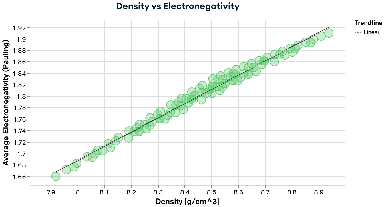
If you are interested in seeing a couple more examples, you can visit the dashboard of ULTERA Database for high entropy alloys.
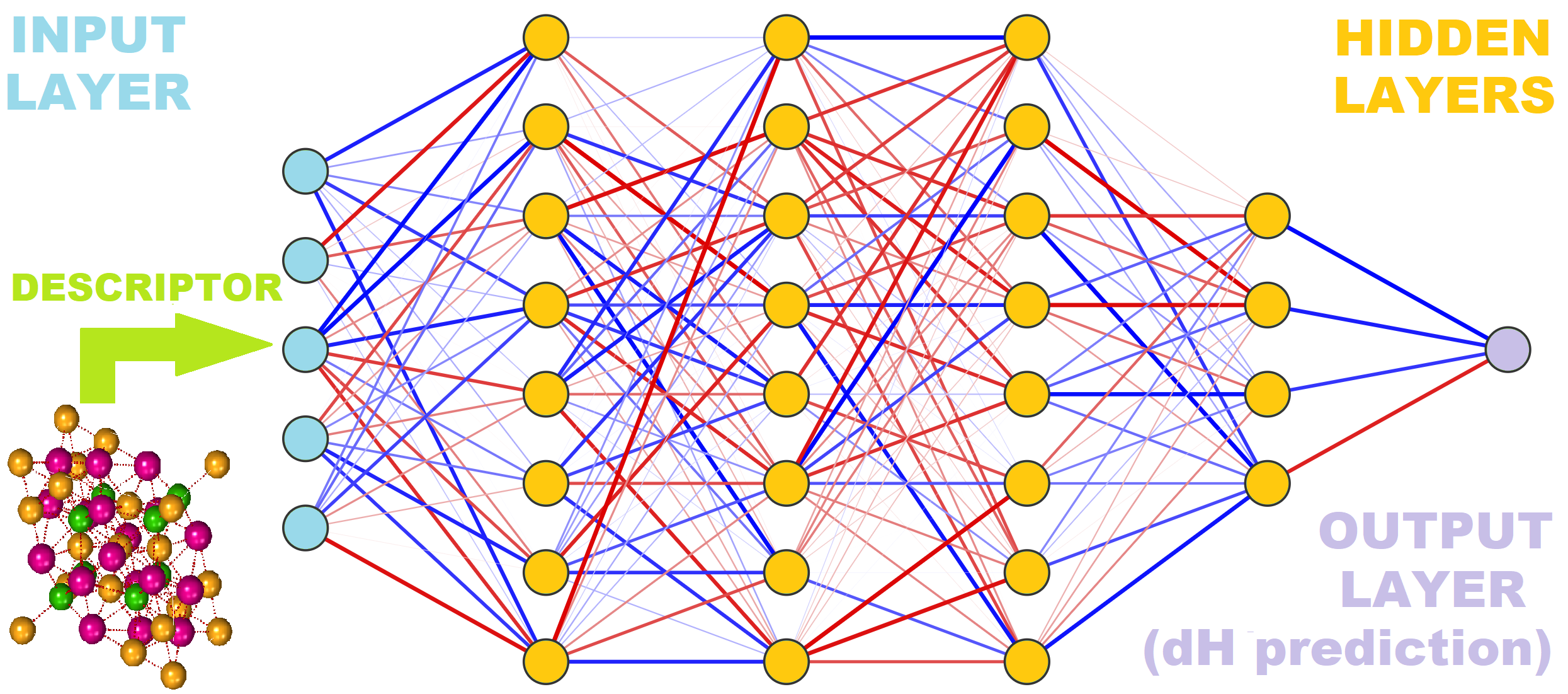
# pySIPFENN
We will now complete a brief walkthrough covering core functionalities of the pySIPFENN or py(Structure-Informed Prediction of Formation Energy using Neural Networks) package; available through the PyPI repository. For a full up-to-date documentation, please refer to the pySIPFENN documentation page or pySIPFENN GitHub repository. You can also find news about our projects using SIPFENN at our Phases Research Lab group website.
On the conceptual level, pySIPFENN is a framework composed of:
-
Featurizers / descriptor calculators allowing the user to interpret atomic structures (hence Structure-Informed) and represent them with numbers in a way suitable for machine learning (ML) Prediction of properties. A few we created are shipped to public; these are Ward2017 (general) and KS2022 (general or optimized to different material types) calcualting Ward2017 and KS2022 feature vectors, respectively. Thanks to how modular pySIPFENN is, you can generally just "steal" them as standalone modules and use them in your own projects.
-
It can handle any properties the user wants to predict based purely on the model training, but the key fundamental property of interest has been Formation Energy of materials, and that is what is shipped by default with the package.
-
It can use any Open Neural Network Exchange (ONNX) trained on the supported feature vectors (Ward2017 and KS2022 included). The models shipped by default are Neural Networks, hence the inclusion in the name, but neither pySIPFENN nor ONNX is limited to NNs. You can export, for instance, complete
scikit-learnpipelines (as done here in heaGAN package) and use them in pySIPFENN.
The figure below shows how they fit together conceptually:
# Getting Started
To utilize pySIPFENN for straightforward calculations, only the Calculator class is needed, which acts as an environment for all package components. Under the hood, it will do many things for you, including both fetching and identification of available NN models. Afterwards, it will expose a very high-level API for you to use.
from pysipfenn import Calculator # The only thing needed for calculations
Could not import coremltools.

Dependencies for exporting to CoreML, Torch, and ONNX are not installed by default with pySIPFENN. You need to install pySIPFENN in "dev" mode like: pip install -e "pysipfenn[dev]", or like pip install -e ".[dev]" ifyou are cloned it. See pysipfenn.org for more details.
Now initialize the Calculator. When run, this should display all models detected (e.g. ✔ SIPFENN_Krajewski2020 Standard Materials Model) and those not detected, but declared in the modelsSIPFENN/models.json file. If some networks are not detected (prepended with x), this may mean the download (you were to do in Lecture 1) was not completed successfully. You can try to download them again by calling c.downloadModels(), which will only download the missing ones.
c = Calculator()
*********  Initializing pySIPFENN Calculator  **********
Loading model definitions from: /Users/adam/opt/anaconda3/envs/580demo/lib/python3.10/site-packages/pysipfenn/modelsSIPFENN/models.json
Found 4 network definitions in models.json
✔ SIPFENN_Krajewski2020 Standard Materials Model
✔ SIPFENN_Krajewski2020 Novel Materials Model
✔ SIPFENN_Krajewski2020 Light Model
✔ SIPFENN_Krajewski2022 KS2022 Novel Materials Model
Loading all available models (autoLoad=True)
Loading models:


100%|██████████| 4/4 [00:13<00:00,  3.27s/it]

*********  pySIPFENN Successfully Initialized  **********
The simplest and most common usage of pySIPFENN is to deploy it on a directory/folder containing atomic structure files such as POSCAR or CIF. To of so, one simply specifies its location and which descriptor / feature vector should be used. The latter determines which ML models will be run, as they require a list of specific and ordered features as input.
c.runFromDirectory(directory='myInputFiles', descriptor='KS2022')
Furthermore, while the exact model can be specified by the user, by default, all applicable models are run, as the run itself is 1-3 orders of magnitude faster than descriptor calculation. Following the link printed during Calculator initialization reveals which models will be run.
In this demonstration, a set of test files shipped under assets/examplePOSCARS. Let's run them with Ward2017 featurizer.
c.runFromDirectory(directory='assets/examplePOSCARS',
                   descriptor='Ward2017');
Importing structures...


100%|██████████| 6/6 [00:00<00:00, 33.33it/s]


Models that will be run: ['SIPFENN_Krajewski2020_NN9', 'SIPFENN_Krajewski2020_NN20', 'SIPFENN_Krajewski2020_NN24']
Calculating descriptors...


100%|██████████| 6/6 [00:04<00:00,  1.35it/s]


Done!
Making predictions...
Prediction rate: 22.0 pred/s
Obtained 6 predictions from:  SIPFENN_Krajewski2020_NN9
Prediction rate: 23.2 pred/s
Obtained 6 predictions from:  SIPFENN_Krajewski2020_NN20
Prediction rate: 132.7 pred/s
Obtained 6 predictions from:  SIPFENN_Krajewski2020_NN24
Done!
Now, all results are obtained and stored within the c Calculator object inside a few exposed conveniently named variables predictions and inputFiles. Also, the descriptor data is retained in descriptorData if needed. Let's look up all 6 entries. Note that the unit of prediction will depend on the model used; in this case, it is eV/atom.
pprint(c.inputFiles)
pprint(c.predictions)
['12-Gd4Cr4O12.POSCAR',
 '13-Fe16Ni14.POSCAR',
 '14-Fe24Ni6.POSCAR',
 '15-Ta4Tl4O12.POSCAR',
 '16-Fe18Ni12.POSCAR',
 '17-Pr4Ga4O12.POSCAR']
[[-3.154766321182251, -3.214848756790161, -3.187128782272339],
 [-0.013867354951798916, 0.04655897989869118, 0.053411152213811874],
 [0.02639671415090561, 0.05997598543763161, 0.06677809357643127],
 [-2.467507839202881, -2.4308743476867676, -2.391871690750122],
 [0.01810809224843979, 0.06462040543556213, 0.10881152749061584],
 [-2.7106518745422363, -2.6583476066589355, -2.727781057357788]]
For user convenience, a few methods are provided for extracting the results. E.g., if pySIPFENN has been run from structure files, the get_resultDictsWithNames() method is available to conveniently pass results forward in the code.
c.get_resultDictsWithNames()
[{'name': '12-Gd4Cr4O12.POSCAR',
  'SIPFENN_Krajewski2020_NN9': -3.154766321182251,
  'SIPFENN_Krajewski2020_NN20': -3.214848756790161,
  'SIPFENN_Krajewski2020_NN24': -3.187128782272339},
 {'name': '13-Fe16Ni14.POSCAR',
  'SIPFENN_Krajewski2020_NN9': -0.013867354951798916,
  'SIPFENN_Krajewski2020_NN20': 0.04655897989869118,
  'SIPFENN_Krajewski2020_NN24': 0.053411152213811874},
 {'name': '14-Fe24Ni6.POSCAR',
  'SIPFENN_Krajewski2020_NN9': 0.02639671415090561,
  'SIPFENN_Krajewski2020_NN20': 0.05997598543763161,
  'SIPFENN_Krajewski2020_NN24': 0.06677809357643127},
 {'name': '15-Ta4Tl4O12.POSCAR',
  'SIPFENN_Krajewski2020_NN9': -2.467507839202881,
  'SIPFENN_Krajewski2020_NN20': -2.4308743476867676,
  'SIPFENN_Krajewski2020_NN24': -2.391871690750122},
 {'name': '16-Fe18Ni12.POSCAR',
  'SIPFENN_Krajewski2020_NN9': 0.01810809224843979,
  'SIPFENN_Krajewski2020_NN20': 0.06462040543556213,
  'SIPFENN_Krajewski2020_NN24': 0.10881152749061584},
 {'name': '17-Pr4Ga4O12.POSCAR',
  'SIPFENN_Krajewski2020_NN9': -2.7106518745422363,
  'SIPFENN_Krajewski2020_NN20': -2.6583476066589355,
  'SIPFENN_Krajewski2020_NN24': -2.727781057357788}]
Alternatively, if results are to be preserved in a spreadsheet, they can be exported into a CSV.
c.writeResultsToCSV('myFirstResults_pySIPFENN.csv')
# Predicting all Sigma Endmembers from Lecture 1
Now, armed with the power of pySIPFENN, we can quickly get the formation energies of all Sigma phase endmembers we defined in Lecture 1. We start by getting all the structures from the database:
structList, idList = [], []
for entry in collection.find({}):
    idList.append(entry['_id'])
    structList.append(Structure.from_dict(entry['structure']))
print(f'Fetched {len(structList)} structures')
Fetched 243 structures
Now, we will use runModels function, which is one layer of abstraction lower than runFromDirectory as it skips file processing and directly takes the structure objects. We will set mode='parallel' to run in parallel, which is much faster than sequential execution on multi-core machines. Each thread on a modern CPU should be able to process ~1 structure per second, so this should take about a minute.
We will also use get_resultDicts to get the results in a convenient format.
c.runModels(structList=structList, descriptor='Ward2017', mode='parallel', max_workers=4)
results = c.get_resultDicts()
Models that will be run: ['SIPFENN_Krajewski2020_NN9', 'SIPFENN_Krajewski2020_NN20', 'SIPFENN_Krajewski2020_NN24']
Calculating descriptors...


  0%|          | 0/243 [00:00<?, ?it/s]


Could not import coremltools.

Could not import coremltools.
Dependencies for exporting to CoreML, Torch, and ONNX are not installed by default with pySIPFENN. You need to install pySIPFENN in "dev" mode like: pip install -e "pysipfenn[dev]", or like pip install -e ".[dev]" ifyou are cloned it. See pysipfenn.org for more details.

Dependencies for exporting to CoreML, Torch, and ONNX are not installed by default with pySIPFENN. You need to install pySIPFENN in "dev" mode like: pip install -e "pysipfenn[dev]", or like pip install -e ".[dev]" ifyou are cloned it. See pysipfenn.org for more details.
Could not import coremltools.

Could not import coremltools.

Dependencies for exporting to CoreML, Torch, and ONNX are not installed by default with pySIPFENN. You need to install pySIPFENN in "dev" mode like: pip install -e "pysipfenn[dev]", or like pip install -e ".[dev]" ifyou are cloned it. See pysipfenn.org for more details.Dependencies for exporting to CoreML, Torch, and ONNX are not installed by default with pySIPFENN. You need to install pySIPFENN in "dev" mode like: pip install -e "pysipfenn[dev]", or like pip install -e ".[dev]" ifyou are cloned it. See pysipfenn.org for more details.

Done!
Making predictions...
Prediction rate: 2442.2 pred/s
Obtained 243 predictions from:  SIPFENN_Krajewski2020_NN9
Prediction rate: 2438.8 pred/s
Obtained 243 predictions from:  SIPFENN_Krajewski2020_NN20
Prediction rate: 13656.1 pred/s
Obtained 243 predictions from:  SIPFENN_Krajewski2020_NN24
pprint(results[0])
{'SIPFENN_Krajewski2020_NN20': 0.07977379858493805,
 'SIPFENN_Krajewski2020_NN24': 0.03619053587317467,
 'SIPFENN_Krajewski2020_NN9': 0.07845475524663925}
and now we can easily upload them back to the database, as we learned in Lecture 1
for id, result in zip(idList, results):
    collection.update_one({'_id': id}, {'$set': result})
and now they are accessible to anyone with access!
collection.find_one({}, skip=100)['SIPFENN_Krajewski2020_NN9']
0.15312525629997253
# Featurization
We've just made some predictions using pySIPFENN and created a dataset to share with the world. Still, like with most ML materials tools, the real power comes from featurization, which is often obfuscated from the user. Fortunately, pySIPFENN is very transparent and allows us to easily access all Ward2017 features for all structures we just predicted under the descriptorData variable of the Calculator object.
print(f'Number of features: {len(c.descriptorData[25])}\nFeature values (first 30):')
pprint(c.descriptorData[25][:30])
print('...\n')
Number of features: 271
Feature values (first 30):
array([12.66417893,  0.56971497, 11.79388959, 13.794477  ,  0.01616931,
        0.96905691,  1.03318127,  0.05207893,  0.01485447,  0.0272743 ,
        0.0661337 ,  0.03462427,  0.20295946,  0.079708  ,  0.03877594,
        0.57907191,  1.58050955,  0.36763378,  1.15612262,  2.83469893,
        1.6785763 ,  4.74152866,  1.10290133,  3.46836787,  8.50409678,
        5.0357289 ,  2.49699209,  0.65083092,  1.7542278 ,  4.93760804])
...
With this data available for all 243 endmembers, we have an embedding of all these structures in so-called feature space. However, it is so highly dimensional that it is impossible to visualize. Fortunately, we can use dimensionality reduction techniques to reduce the number of dimensions to 2 or 3 and visualize the results for human eyes.
We will use TSNE (t-distributed stochastic neighbor embedding) to reduce the dimensionality to 2 using the sklearn library. It is not a part of pySIPFENN dependency tree, so you may need to install it with pip below (after uncommenting the line).
#!pip install scikit-learn
from sklearn.manifold import TSNE              # neighborhood  dimensionality reduction
from sklearn.preprocessing import MinMaxScaler # scaling
We start by copying the c.descriptorData, normalizing it across feature values to minima and maxima using MinMaxScaler (similar to fixed Max scaler inside pySIPFENN NNs), and setting up the TSNE object.
scaler = MinMaxScaler()
descriptorData = scaler.fit_transform(np.array(c.descriptorData))
We will use perplexity=4, as we don't expect large clusters, n_iter=1000 to speed up the calculation, the pca initialization to give a good starting point, and use
scipy.spatial.distance.correlation as the neighbor distance metric between points.
You are certainly encouraged to play with these parameters to see how they affect the results!
tsne = TSNE(n_components=2, perplexity=4, init='pca', n_iter=2000, metric='correlation', angle=0.2, n_jobs=-1)
Now, let's embed the data in 2D space and look at the first 5 results as a sanity check.
embeddedDescriptorData = tsne.fit_transform(descriptorData)
pprint(embeddedDescriptorData[:5])
array([[ 41.368214, -60.807182],
       [-22.270252,  72.0951  ],
       [ 45.874958, -56.52266 ],
       [-25.202972,  67.837654],
       [-31.33803 ,  58.68771 ]], dtype=float32)
Note that the embedding is stochastic and chaotic, so you will get different results each time you run it. However, you can easily fix it by setting the random_state parameter to a fixed value of 580. Note: this value will persist across the notebook now.
tsne.random_state = 580
embeddedDescriptorData = tsne.fit_transform(descriptorData)
pprint(embeddedDescriptorData[:5])
array([[ 41.368214, -60.807182],
       [-22.270252,  72.0951  ],
       [ 45.874958, -56.52266 ],
       [-25.202972,  67.837654],
       [-31.33803 ,  58.68771 ]], dtype=float32)
Finally, we can plot the results using plotly library. We will colorize the points by the formation energy coming from the first model in c.predictions variable. We will also use structList to get chemical formulas when hovering over the points.
fig = px.scatter(x=np.transpose(embeddedDescriptorData)[0],
                 y=np.transpose(embeddedDescriptorData)[1],
                 hover_name=[s.formula for s in structList],
                 color=[round(p[0], 3) for p in c.predictions],
                 color_discrete_sequence=px.colors.qualitative.Dark24,
                 template='plotly_white',
                 labels={'x': f'{len(descriptorData[0])}D->2D TSNE1',
                         'y': f'{len(descriptorData[0])}D->2D TSNE2',
                         'color': f'Formation Energy (eV/atom)'},
                 height=400,
                 width=800
                 )
fig.show()

An immediate result one can see here is that similar structures in the feature space have similar energies in the prediction space, which is a good sign that the method is working as expected.
Before moving further, let's upload the results to the database so we can visualize them later in MongoDB Charts if we want to.
for id, embedding in zip(idList, embeddedDescriptorData.tolist()):
    collection.update_one(
        {'_id': id},
        {'$set': {'TSNE_2D_X': embedding[0], 'TSNE_2D_Y': embedding[1]}})
Next, ley's check how the data looks like. For clarity, we can ask pymongo to skip part of the data entry in a process called projection by setting it to 0 in a dictionary of fields directly after the query. In this case, we are skipping the structure and POSCAR fields.
collection.find_one({}, {'structure': 0, 'POSCAR': 0}, skip=100)
{'_id': ObjectId('6531516032703fc61d08d457'),
 'composition': {'Cr': 12.0, 'Fe': 10.0, 'Ni': 8.0},
 'density': 8.38605032076435,
 'reducedFormula': 'Cr6Fe5Ni4',
 'weightFractions': {'Cr': 0.37770698200139663,
  'Fe': 0.33805494402253244,
  'Ni': 0.2842380739760709},
 'permutation': 'CrFeNiFeCr',
 'autor': 'Happy Student',
 'creationDate': datetime.datetime(2023, 10, 19, 15, 55, 12, 965000),
 'averageElectronegativity': 1.7833333333333334,
 'SIPFENN_Krajewski2020_NN20': 0.1178784966468811,
 'SIPFENN_Krajewski2020_NN24': 0.11623784899711609,
 'SIPFENN_Krajewski2020_NN9': 0.15312525629997253,
 'TSNE_2D_X': 22.739927291870117,
 'TSNE_2D_Y': 63.28989028930664,
 'DFT_dH': 0.103503167}
# Transfer Learning on small DFT dataset
Now, let's look at an example of how we can use this data to guide DFT calculations!
There are a few possible ways, but we will focus on transfer learning, which is a technique of using a model trained on a large dataset (e.g. all OQMD, like NN20 we used, or Materials Project) and fine-tuning it on a smaller dataset (e.g. 10 DFT calculations of Sigma phase endmembers).
dftN = 12
# Selecting a subset of data
The most critical step to getting good performance here is the selection of a good small subset we will train on.
This can be done in many ways, but the baseline is a random selection like:
import random

randomEndmembersList = random.sample(range(len(descriptorData)), dftN)
print(randomEndmembersList)
[76, 79, 189, 45, 195, 124, 219, 112, 6, 186, 86, 75]
However, with the feature space embedding, we can on average do better than that! Let's look for some representative structures in the feature space by identifying cluster centers with KMeans clustering from, again, sklearn library, and locating points nearest to them by computing pairwise_distances matrix between all points and cluster centers.
from sklearn.cluster import KMeans                          # clustering method
from sklearn.metrics import pairwise_distances_argmin_min   # distance metric

kmeansClustering = KMeans(n_clusters=dftN, n_init=500, max_iter=1000, random_state=580)
clusterData = kmeansClustering.fit(embeddedDescriptorData)
print(clusterData.cluster_centers_)
[[-64.198555   -38.431873  ]
 [-12.584402    12.041971  ]
 [ 51.93679     41.060352  ]
 [ 52.304935   -50.383396  ]
 [-14.359932   -48.381523  ]
 [-27.307589    65.01916   ]
 [-68.85164     23.871618  ]
 [ 67.888756     9.928222  ]
 [ 10.148277     0.46234655]
 [ 30.642172    57.845394  ]
 [-42.25075    -30.75432   ]
 [ 31.958817   -69.17891   ]]
clusterCenters, _ = pairwise_distances_argmin_min(clusterData.cluster_centers_, embeddedDescriptorData)
print(clusterCenters)
[ 89 219 14 216 239 108 13 124 63 156 25 182]
which we can now plot on top of the TSNE embedding we made earlier.
fig = px.scatter(x=np.transpose(embeddedDescriptorData)[0],
                 y=np.transpose(embeddedDescriptorData)[1],
                 hover_name=[s.formula for s in structList],
                 color=['cluster center' if i in clusterCenters else 'other' for i in
                        range(len(embeddedDescriptorData))],
                 opacity=0.85,
                 color_discrete_sequence=px.colors.qualitative.Dark24,
                 template='plotly_white',
                 labels={'x': f'{len(descriptorData[0])}D->2D TSNE1',
                         'y': f'{len(descriptorData[0])}D->2D TSNE2',
                         'color': f'Embedded Points'},
                 height=400,
                 width=800
                 )
fig.show()

# Our virtual HPC Run
Before we go forward, in order to prove that a selection of points for DFT was good, we need to calculate all of them, even though only a small subset will be used for training.
To do so, we will now take results pre-calculated with DFTTK (in assets/sigma.csv) and insert them into the database; pretending they were calculated on a HPC cluster. The result will be functionally the same.
Note we will be matching them by permutation (with the same order of elements we used earlier) and not by the id as we did earlier, since the order of results is not guaranteed to be the same.
with open('assets/sigma.csv', 'r') as sigmaData:
    for l in sigmaData.readlines()[1:]:
        lSplit = l.split(',')
        permutation = "".join(lSplit[0:5])
        DFT_dH = float(lSplit[8])
        collection.update_one({'permutation': permutation}, {'$set': {'DFT_dH': DFT_dH}})
collection.find_one({}, {'structure': 0, 'POSCAR': 0}, skip=100)
{'_id': ObjectId('6531516032703fc61d08d457'),
 'composition': {'Cr': 12.0, 'Fe': 10.0, 'Ni': 8.0},
 'density': 8.38605032076435,
 'reducedFormula': 'Cr6Fe5Ni4',
 'weightFractions': {'Cr': 0.37770698200139663,
  'Fe': 0.33805494402253244,
  'Ni': 0.2842380739760709},
 'permutation': 'CrFeNiFeCr',
 'autor': 'Happy Student',
 'creationDate': datetime.datetime(2023, 10, 19, 15, 55, 12, 965000),
 'averageElectronegativity': 1.7833333333333334,
 'SIPFENN_Krajewski2020_NN20': 0.1178784966468811,
 'SIPFENN_Krajewski2020_NN24': 0.11623784899711609,
 'SIPFENN_Krajewski2020_NN9': 0.15312525629997253,
 'TSNE_2D_X': 22.739927291870117,
 'TSNE_2D_Y': 63.28989028930664,
 'DFT_dH': 0.103503167}
# Fine-Tuning the Models
Now, we are ready to fine-tune the models! In the (near) future release of pySIPFENN, this will be done using a high-level API (including hyperparameter tuning); thus, if you are following this lecture in the future, you may want to check out the documentation for the latest version. For now, we will do it manually by calling many torch and onnx functions, which won't be explained in this lecture, but I am happy to discuss them during office hours.
If you are interested in learning more about what we are doing here, you can have a look at Section 3.5 in the SIPFENN paper.
import torch
import onnx
import onnx2torch
import random
Pull DFT data from the database and convert it to a torch tensor. The {'DFT_dH': 1} after the query is a projection, which means we only want to get the DFT_dH field from the database. This is a good practice to reduce the amount of data transferred over the network.
labelTensor = torch.from_numpy(np.array([[collection.find_one({'_id': id}, {'DFT_dH': 1})['DFT_dH']] for id in idList])).float()
print(labelTensor[:10])
tensor([[0.0805],
        [0.0778],
        [0.0802],
        [0.0935],
        [0.0809],
        [0.1118],
        [0.0656],
        [0.0678],
        [0.0702],
        [0.0867]])
Convert the numpy array to torch tensor.
ddTensor = torch.from_numpy(descriptorData).float()
Load the underlying model, in this case NN24 as it is the lightest on memory and fasterst to tune, and get it ready. Alternatively, you could use loadedModels from c by copying them with copy.deepcopy, but that would be slower and use more memory than necessary.
with resources.files('pysipfenn').joinpath('modelsSIPFENN/SIPFENN_Krajewski2020_NN24.onnx') as nn24model:
    model = onnx2torch.convert(onnx.load(nn24model))
    model.eval()
Set the optimizer and MAE loss function.
optimizer = torch.optim.Adam(model.parameters(), lr=0.00005)
loss = torch.nn.L1Loss()
And before we go further, let's see the current performance of the model on the DFT data we just pulled.
dataOut = model(ddTensor, None)
print(dataOut[:10])
tensor([[ 0.1671],
        [ 0.3394],
        [ 0.1794],
        [ 0.5271],
        [ 0.4225],
        [ 0.4708],
        [ 0.2241],
        [ 0.4732],
        [-0.2594],
        [ 0.4692]], grad_fn=<SliceBackward0>)
loss(dataOut, labelTensor)
tensor(0.2319, grad_fn=<MeanBackward0>)
# Random Selection
Randomly select the subset of data to train on.
transferIndexes = random.sample(range(len(descriptorData)), dftN)
validationIndexes = list(set(range(len(descriptorData))).difference(transferIndexes))
print(transferIndexes)
[76, 190, 11, 0, 84, 218, 87, 219, 79, 52, 164, 26]
Cherry-pick the data creating new tensors
transferData = torch.index_select(ddTensor, 0, torch.LongTensor(transferIndexes)).float()
transferLabels = torch.index_select(labelTensor, 0, torch.LongTensor(transferIndexes)).float()

validationData = torch.index_select(ddTensor, 0, torch.LongTensor(validationIndexes)).float()
validationLabels = torch.index_select(labelTensor, 0, torch.LongTensor(validationIndexes)).float()
And finally, train the model!
model.eval()
transferLosses = [float(loss(model(transferData, None), transferLabels))]
validationLosses = [float(loss(model(validationData, None), validationLabels))]

model.train()
print('Initial Mean Absolute Errors (MAE):')
print(f'Train: {round(1000 * float(transferLosses[0]), 1):>5}  |  Val: {round(1000 * float(validationLosses[0]), 1):>5}   [meV/atom]')
print('Starting Training...')
for i in range(250):
    optimizer.zero_grad()
    transfer_pred = model(transferData, None)
    transfer_loss = loss(transfer_pred, transferLabels)
    transferLosses.append(float(transfer_loss))
    transfer_loss.backward()
    optimizer.step()
    validationLosses.append(float(loss(model(validationData, None), validationLabels)))
    if i % 10 == 0:
        print(f'Epoch {i:>3}:  Train: {round(1000 * float(transferLosses[-1]), 1):>5}  |  Val: {round(1000 * float(validationLosses[-1]), 1):>5}   [meV/atom]')
print('Training Complete!')
model.eval()
transferLosses.append(float(loss(model(transferData, None), transferLabels)))
validationLosses.append(float(loss(model(validationData, None), validationLabels)))
print('Final Evaluation Mean Absolute Error (MAE):')
print(f'Train: {round(1000 * float(transferLosses[-1]), 1):>5}  |  Val: {round(1000 * float(validationLosses[-1]), 1):>5}')
Initial Mean Absolute Errors (MAE):
Train: 263.6  |  Val: 230.2   [meV/atom]
Starting Training...
Epoch   0:  Train: 266.0  |  Val: 202.5   [meV/atom]
Epoch  10:  Train:  86.8  |  Val: 124.6   [meV/atom]
Epoch  20:  Train:  53.9  |  Val: 100.7   [meV/atom]
Epoch  30:  Train:  37.8  |  Val:  69.9   [meV/atom]
Epoch  40:  Train:  33.1  |  Val:  63.9   [meV/atom]
Epoch  50:  Train:  24.9  |  Val:  56.0   [meV/atom]
Epoch  60:  Train:  20.0  |  Val:  56.6   [meV/atom]
Epoch  70:  Train:  25.9  |  Val:  53.5   [meV/atom]
Epoch  80:  Train:  19.7  |  Val:  50.4   [meV/atom]
Epoch  90:  Train:  23.4  |  Val:  45.9   [meV/atom]
Epoch 100:  Train:  19.4  |  Val:  48.1   [meV/atom]
Epoch 110:  Train:  35.5  |  Val:  44.9   [meV/atom]
Epoch 120:  Train:  21.7  |  Val:  45.4   [meV/atom]
Epoch 130:  Train:  13.4  |  Val:  42.8   [meV/atom]
Epoch 140:  Train:  20.2  |  Val:  38.7   [meV/atom]
Epoch 150:  Train:  13.2  |  Val:  44.2   [meV/atom]
Epoch 160:  Train:  17.0  |  Val:  39.5   [meV/atom]
Epoch 170:  Train:  14.5  |  Val:  38.7   [meV/atom]
Epoch 180:  Train:  21.5  |  Val:  38.9   [meV/atom]
Epoch 190:  Train:  15.2  |  Val:  38.8   [meV/atom]
Epoch 200:  Train:  12.5  |  Val:  38.1   [meV/atom]
Epoch 210:  Train:  12.6  |  Val:  38.7   [meV/atom]
Epoch 220:  Train:  12.9  |  Val:  39.5   [meV/atom]
Epoch 230:  Train:  19.4  |  Val:  36.4   [meV/atom]
Epoch 240:  Train:  15.2  |  Val:  38.2   [meV/atom]
Training Complete!
Final Evaluation Mean Absolute Error (MAE):
Train:   6.8  |  Val:  30.1
# Feature-Space-Informed Selection
Now, lets do the same, but using the subset of data we selected based on the feature space embedding and assigned to clusterCenters variable.
Start by reloading feature data from pySIPFENN.
with resources.files('pysipfenn').joinpath('modelsSIPFENN/SIPFENN_Krajewski2020_NN24.onnx') as nn24model:
    model = onnx2torch.convert(onnx.load(nn24model))
    model.eval()

optimizer = torch.optim.Adam(model.parameters(), lr=0.00005)
loss = torch.nn.L1Loss()
Select the subset with clusterCenters and convert it to torch tensor.
transferIndexes = clusterCenters
validationIndexes = list(set(range(len(descriptorData))).difference(clusterCenters))
print(transferIndexes)
[ 89 219 14 216 239 108 13 124 63 156 25 182]
transferData = torch.index_select(ddTensor, 0, torch.LongTensor(transferIndexes)).float()
transferLabels = torch.index_select(labelTensor, 0, torch.LongTensor(transferIndexes)).float()

validationData = torch.index_select(ddTensor, 0, torch.LongTensor(validationIndexes)).float()
validationLabels = torch.index_select(labelTensor, 0, torch.LongTensor(validationIndexes)).float()
model.eval()
transferLosses = [float(loss(model(transferData, None), transferLabels))]
validationLosses = [float(loss(model(validationData, None), validationLabels))]

model.train()
print('Initial Mean Absolute Errors (MAE):')
print(f'Train: {round(1000 * float(transferLosses[0]), 1):>5}  |  Val: {round(1000 * float(validationLosses[0]), 1):>5}   [meV/atom]')
print('Starting Training...')
for i in range(250):
    optimizer.zero_grad()
    transfer_pred = model(transferData, None)
    transfer_loss = loss(transfer_pred, transferLabels)
    transferLosses.append(float(transfer_loss))
    transfer_loss.backward()
    optimizer.step()
    validationLosses.append(float(loss(model(validationData, None), validationLabels)))
    if i % 10 == 0:
        print(f'Epoch {i:>3}:  Train: {round(1000 * float(transferLosses[-1]), 1):>5}  |  Val: {round(1000 * float(validationLosses[-1]), 1):>5}')
print('Training Complete!')
model.eval()
transferLosses.append(float(loss(model(transferData, None), transferLabels)))
validationLosses.append(float(loss(model(validationData, None), validationLabels)))
print('Final Evaluation Mean Absolute Error (MAE):')
print(f'Train: {round(1000 * float(transferLosses[-1]), 1):>5}  |  Val: {round(1000 * float(validationLosses[-1]), 1):>5}')
Initial Mean Absolute Errors (MAE):
Train: 266.1  |  Val: 230.1   [meV/atom]
Starting Training...
Epoch   0:  Train: 297.3  |  Val: 202.5
Epoch  10:  Train: 121.2  |  Val: 118.8
Epoch  20:  Train:  20.9  |  Val:  76.5
Epoch  30:  Train:  35.6  |  Val:  56.4
Epoch  40:  Train:  40.7  |  Val:  50.5
Epoch  50:  Train:  33.6  |  Val:  48.2
Epoch  60:  Train:  31.6  |  Val:  45.6
Epoch  70:  Train:  25.6  |  Val:  42.3
Epoch  80:  Train:  29.8  |  Val:  43.7
Epoch  90:  Train:  20.5  |  Val:  41.7
Epoch 100:  Train:  23.3  |  Val:  41.8
Epoch 110:  Train:  13.6  |  Val:  41.6
Epoch 120:  Train:  18.4  |  Val:  35.7
Epoch 130:  Train:  20.6  |  Val:  38.5
Epoch 140:  Train:  15.7  |  Val:  34.5
Epoch 150:  Train:  17.5  |  Val:  32.5
Epoch 160:  Train:  20.6  |  Val:  33.3
Epoch 170:  Train:  17.3  |  Val:  36.0
Epoch 180:  Train:  12.2  |  Val:  30.6
Epoch 190:  Train:  17.3  |  Val:  31.9
Epoch 200:  Train:  17.4  |  Val:  29.5
Epoch 210:  Train:  16.2  |  Val:  30.0
Epoch 220:  Train:  11.7  |  Val:  30.5
Epoch 230:  Train:   8.4  |  Val:  28.3
Epoch 240:  Train:  13.9  |  Val:  32.8
Training Complete!
Final Evaluation Mean Absolute Error (MAE):
Train:   9.5  |  Val:  26.3
Now, on average you should see a result around 25meV/atom depending on the run, which should be around 20-30% reduction in MAE, which is a significant improvement! However, the real power of this approach lays in its consistency, as if you repeat this process many times, the random selection may sometimes happen to be better, but it will ocassionally be two or three times higher.
# Conclusions and Further Resources
If you were able to complete this notebook, you should now have a good basic understanding of how manipulte atomic configurations in Python, send it back and forth to MongoDB, and use pySIPFENN to (1) predict formation energy, (2) featurize structures, and (3) tune ML models.
Here are some additional resources you may find useful if you want to learn more:
- MongoDB Compass GUI Application which will allow you to interact with the database in a very user-friendly way, including basic visualization of the data, testing your queries, analyzing the structure of the database, and more.
- MongoDB Query Language (MQL) documentation
- pySIPFENN documentation and pySIPFENN GitHub repository
- Results section of SIPFENN Paper for a discussion of how and why we do transfer learning. Including reasoning behing some hyperparameters we used here.